Predicting interest rates at the Lending Club

Introduction
The goal of this analysis is to walk through the mechanics of designing a predictive model using linear regression. The example we will use is Lending Club, a peer-to-peer lender. The goal is to come up with an algorithm that recommends the interest rate to charge to new loans. The lending club has made historical data publicly available and we will use it for this exercise.
Load and prepare the data
We start by loading the data to R in a dataframe.
lc_raw <- read_csv(here::here("data", "LendingClub Data.csv"), skip=1) %>%  #since the first row is a title we want to skip it.
  clean_names() # use janitor::clean_names()
ICE the data: Inspect, Clean, Explore
Any data science engagement starts with ICE. Inspect, Clean and Explore the data.
glimpse(lc_raw) ## Rows: 42,538
## Columns: 80
## $ int_rate <dbl> 0.05, 0.05, 0.05, 0.05, 0.05, 0.05, 0.05, 0.05, 0…
## $ loan_amnt <dbl> 8000, 6000, 6500, 8000, 5500, 6000, 10200, 15000,…
## $ term_months <dbl> 36, 36, 36, 36, 36, 36, 36, 36, 36, 36, 36, 36, 3…
## $ installment <dbl> 241.28, 180.96, 196.04, 241.28, 165.88, 180.96, 3…
## $ dti <dbl> 2.11, 5.73, 17.68, 22.71, 5.75, 21.92, 18.62, 9.7…
## $ delinq_2yrs <dbl> 0, 0, 0, 0, 0, 0, 0, 0, 0, 0, 0, 0, 0, 0, 0, 0, 0…
## $ annual_inc <dbl> 50000, 52800, 35352, 79200, 240000, 89000, 110000…
## $ grade <chr> "A", "A", "A", "A", "A", "A", "A", "A", "A", "A",…
## $ emp_title <chr> NA, "coral graphics", NA, "Honeywell", "O T Plus,…
## $ emp_length <chr> "5 years", "< 1 year", "n/a", "n/a", "10+ years",…
## $ home_ownership <chr> "MORTGAGE", "MORTGAGE", "MORTGAGE", "MORTGAGE", "…
## $ verification_status <chr> "Verified", "Source Verified", "Not Verified", "V…
## $ issue_d <chr> "9/1/2011", "9/1/2011", "9/1/2011", "9/1/2011", "…
## $ zip_code <chr> "977xx", "228xx", "864xx", "322xx", "278xx", "760…
## $ addr_state <chr> "OR", "VA", "AZ", "FL", "NC", "TX", "CT", "WA", "…
## $ loan_status <chr> "Fully Paid", "Charged Off", "Fully Paid", "Fully…
## $ desc <chr> "Borrower added on 09/08/11 > Consolidating debt …
## $ purpose <chr> "debt_consolidation", "vacation", "credit_card", …
## $ title <chr> "Credit Card Payoff $8K", "bad choice", "Credit C…
## $ x20 <lgl> NA, NA, NA, NA, NA, NA, NA, NA, NA, NA, NA, NA, N…
## $ x21 <lgl> NA, NA, NA, NA, NA, NA, NA, NA, NA, NA, NA, NA, N…
## $ x22 <lgl> NA, NA, NA, NA, NA, NA, NA, NA, NA, NA, NA, NA, N…
## $ x23 <lgl> NA, NA, NA, NA, NA, NA, NA, NA, NA, NA, NA, NA, N…
## $ x24 <lgl> NA, NA, NA, NA, NA, NA, NA, NA, NA, NA, NA, NA, N…
## $ x25 <lgl> NA, NA, NA, NA, NA, NA, NA, NA, NA, NA, NA, NA, N…
## $ x26 <lgl> NA, NA, NA, NA, NA, NA, NA, NA, NA, NA, NA, NA, N…
## $ x27 <lgl> NA, NA, NA, NA, NA, NA, NA, NA, NA, NA, NA, NA, N…
## $ x28 <lgl> NA, NA, NA, NA, NA, NA, NA, NA, NA, NA, NA, NA, N…
## $ x29 <lgl> NA, NA, NA, NA, NA, NA, NA, NA, NA, NA, NA, NA, N…
## $ x30 <lgl> NA, NA, NA, NA, NA, NA, NA, NA, NA, NA, NA, NA, N…
## $ x31 <lgl> NA, NA, NA, NA, NA, NA, NA, NA, NA, NA, NA, NA, N…
## $ x32 <lgl> NA, NA, NA, NA, NA, NA, NA, NA, NA, NA, NA, NA, N…
## $ x33 <lgl> NA, NA, NA, NA, NA, NA, NA, NA, NA, NA, NA, NA, N…
## $ x34 <lgl> NA, NA, NA, NA, NA, NA, NA, NA, NA, NA, NA, NA, N…
## $ x35 <lgl> NA, NA, NA, NA, NA, NA, NA, NA, NA, NA, NA, NA, N…
## $ x36 <lgl> NA, NA, NA, NA, NA, NA, NA, NA, NA, NA, NA, NA, N…
## $ x37 <lgl> NA, NA, NA, NA, NA, NA, NA, NA, NA, NA, NA, NA, N…
## $ x38 <lgl> NA, NA, NA, NA, NA, NA, NA, NA, NA, NA, NA, NA, N…
## $ x39 <lgl> NA, NA, NA, NA, NA, NA, NA, NA, NA, NA, NA, NA, N…
## $ x40 <lgl> NA, NA, NA, NA, NA, NA, NA, NA, NA, NA, NA, NA, N…
## $ x41 <lgl> NA, NA, NA, NA, NA, NA, NA, NA, NA, NA, NA, NA, N…
## $ x42 <lgl> NA, NA, NA, NA, NA, NA, NA, NA, NA, NA, NA, NA, N…
## $ x43 <lgl> NA, NA, NA, NA, NA, NA, NA, NA, NA, NA, NA, NA, N…
## $ x44 <lgl> NA, NA, NA, NA, NA, NA, NA, NA, NA, NA, NA, NA, N…
## $ x45 <lgl> NA, NA, NA, NA, NA, NA, NA, NA, NA, NA, NA, NA, N…
## $ x46 <lgl> NA, NA, NA, NA, NA, NA, NA, NA, NA, NA, NA, NA, N…
## $ x47 <lgl> NA, NA, NA, NA, NA, NA, NA, NA, NA, NA, NA, NA, N…
## $ x48 <lgl> NA, NA, NA, NA, NA, NA, NA, NA, NA, NA, NA, NA, N…
## $ x49 <lgl> NA, NA, NA, NA, NA, NA, NA, NA, NA, NA, NA, NA, N…
## $ x50 <lgl> NA, NA, NA, NA, NA, NA, NA, NA, NA, NA, NA, NA, N…
## $ x51 <lgl> NA, NA, NA, NA, NA, NA, NA, NA, NA, NA, NA, NA, N…
## $ x52 <lgl> NA, NA, NA, NA, NA, NA, NA, NA, NA, NA, NA, NA, N…
## $ x53 <lgl> NA, NA, NA, NA, NA, NA, NA, NA, NA, NA, NA, NA, N…
## $ x54 <lgl> NA, NA, NA, NA, NA, NA, NA, NA, NA, NA, NA, NA, N…
## $ x55 <lgl> NA, NA, NA, NA, NA, NA, NA, NA, NA, NA, NA, NA, N…
## $ x56 <lgl> NA, NA, NA, NA, NA, NA, NA, NA, NA, NA, NA, NA, N…
## $ x57 <lgl> NA, NA, NA, NA, NA, NA, NA, NA, NA, NA, NA, NA, N…
## $ x58 <lgl> NA, NA, NA, NA, NA, NA, NA, NA, NA, NA, NA, NA, N…
## $ x59 <lgl> NA, NA, NA, NA, NA, NA, NA, NA, NA, NA, NA, NA, N…
## $ x60 <lgl> NA, NA, NA, NA, NA, NA, NA, NA, NA, NA, NA, NA, N…
## $ x61 <lgl> NA, NA, NA, NA, NA, NA, NA, NA, NA, NA, NA, NA, N…
## $ x62 <lgl> NA, NA, NA, NA, NA, NA, NA, NA, NA, NA, NA, NA, N…
## $ x63 <lgl> NA, NA, NA, NA, NA, NA, NA, NA, NA, NA, NA, NA, N…
## $ x64 <lgl> NA, NA, NA, NA, NA, NA, NA, NA, NA, NA, NA, NA, N…
## $ x65 <lgl> NA, NA, NA, NA, NA, NA, NA, NA, NA, NA, NA, NA, N…
## $ x66 <lgl> NA, NA, NA, NA, NA, NA, NA, NA, NA, NA, NA, NA, N…
## $ x67 <lgl> NA, NA, NA, NA, NA, NA, NA, NA, NA, NA, NA, NA, N…
## $ x68 <lgl> NA, NA, NA, NA, NA, NA, NA, NA, NA, NA, NA, NA, N…
## $ x69 <lgl> NA, NA, NA, NA, NA, NA, NA, NA, NA, NA, NA, NA, N…
## $ x70 <lgl> NA, NA, NA, NA, NA, NA, NA, NA, NA, NA, NA, NA, N…
## $ x71 <lgl> NA, NA, NA, NA, NA, NA, NA, NA, NA, NA, NA, NA, N…
## $ x72 <lgl> NA, NA, NA, NA, NA, NA, NA, NA, NA, NA, NA, NA, N…
## $ x73 <lgl> NA, NA, NA, NA, NA, NA, NA, NA, NA, NA, NA, NA, N…
## $ x74 <lgl> NA, NA, NA, NA, NA, NA, NA, NA, NA, NA, NA, NA, N…
## $ x75 <lgl> NA, NA, NA, NA, NA, NA, NA, NA, NA, NA, NA, NA, N…
## $ x76 <lgl> NA, NA, NA, NA, NA, NA, NA, NA, NA, NA, NA, NA, N…
## $ x77 <lgl> NA, NA, NA, NA, NA, NA, NA, NA, NA, NA, NA, NA, N…
## $ x78 <lgl> NA, NA, NA, NA, NA, NA, NA, NA, NA, NA, NA, NA, N…
## $ x79 <lgl> NA, NA, NA, NA, NA, NA, NA, NA, NA, NA, NA, NA, N…
## $ x80 <lgl> NA, NA, NA, NA, NA, NA, NA, NA, NA, NA, NA, NA, N…lc_clean<- lc_raw %>%
dplyr::select(-x20:-x80) %>% #delete empty columns
filter(!is.na(int_rate)) %>% #delete empty rows
mutate(
issue_d = mdy(issue_d), # lubridate::mdy() to fix date format
term = factor(term_months), # turn 'term' into a categorical variable
delinq_2yrs = factor(delinq_2yrs) # turn 'delinq_2yrs' into a categorical variable
) %>%
dplyr::select(-emp_title,-installment, -term_months, everything()) #move some not-so-important variables to the end.
glimpse(lc_clean) ## Rows: 37,869
## Columns: 20
## $ int_rate <dbl> 0.05, 0.05, 0.05, 0.05, 0.05, 0.05, 0.05, 0.05, 0…
## $ loan_amnt <dbl> 8000, 6000, 6500, 8000, 5500, 6000, 10200, 15000,…
## $ dti <dbl> 2.11, 5.73, 17.68, 22.71, 5.75, 21.92, 18.62, 9.7…
## $ delinq_2yrs <fct> 0, 0, 0, 0, 0, 0, 0, 0, 0, 0, 0, 0, 0, 0, 0, 0, 0…
## $ annual_inc <dbl> 50000, 52800, 35352, 79200, 240000, 89000, 110000…
## $ grade <chr> "A", "A", "A", "A", "A", "A", "A", "A", "A", "A",…
## $ emp_length <chr> "5 years", "< 1 year", "n/a", "n/a", "10+ years",…
## $ home_ownership <chr> "MORTGAGE", "MORTGAGE", "MORTGAGE", "MORTGAGE", "…
## $ verification_status <chr> "Verified", "Source Verified", "Not Verified", "V…
## $ issue_d <date> 2011-09-01, 2011-09-01, 2011-09-01, 2011-09-01, …
## $ zip_code <chr> "977xx", "228xx", "864xx", "322xx", "278xx", "760…
## $ addr_state <chr> "OR", "VA", "AZ", "FL", "NC", "TX", "CT", "WA", "…
## $ loan_status <chr> "Fully Paid", "Charged Off", "Fully Paid", "Fully…
## $ desc <chr> "Borrower added on 09/08/11 > Consolidating debt …
## $ purpose <chr> "debt_consolidation", "vacation", "credit_card", …
## $ title <chr> "Credit Card Payoff $8K", "bad choice", "Credit C…
## $ term <fct> 36, 36, 36, 36, 36, 36, 36, 36, 36, 36, 36, 36, 3…
## $ term_months <dbl> 36, 36, 36, 36, 36, 36, 36, 36, 36, 36, 36, 36, 3…
## $ installment <dbl> 241.28, 180.96, 196.04, 241.28, 165.88, 180.96, 3…
## $ emp_title <chr> NA, "coral graphics", NA, "Honeywell", "O T Plus,…The data is now in a clean format stored in the dataframe “lc_clean.”
Exploring the data with some visualizations.
#  Histogram of interest rates.
ggplot(lc_clean, aes(x=int_rate))+
  geom_histogram(binwidth = 0.01)+
  theme_bw()+
  scale_x_continuous(labels=scales::percent)+
  theme(legend.position = "none")+
  labs(
    title = "Interest Rate Distribution",
    x= "Interest Rate",
    y="Count")+
  NULL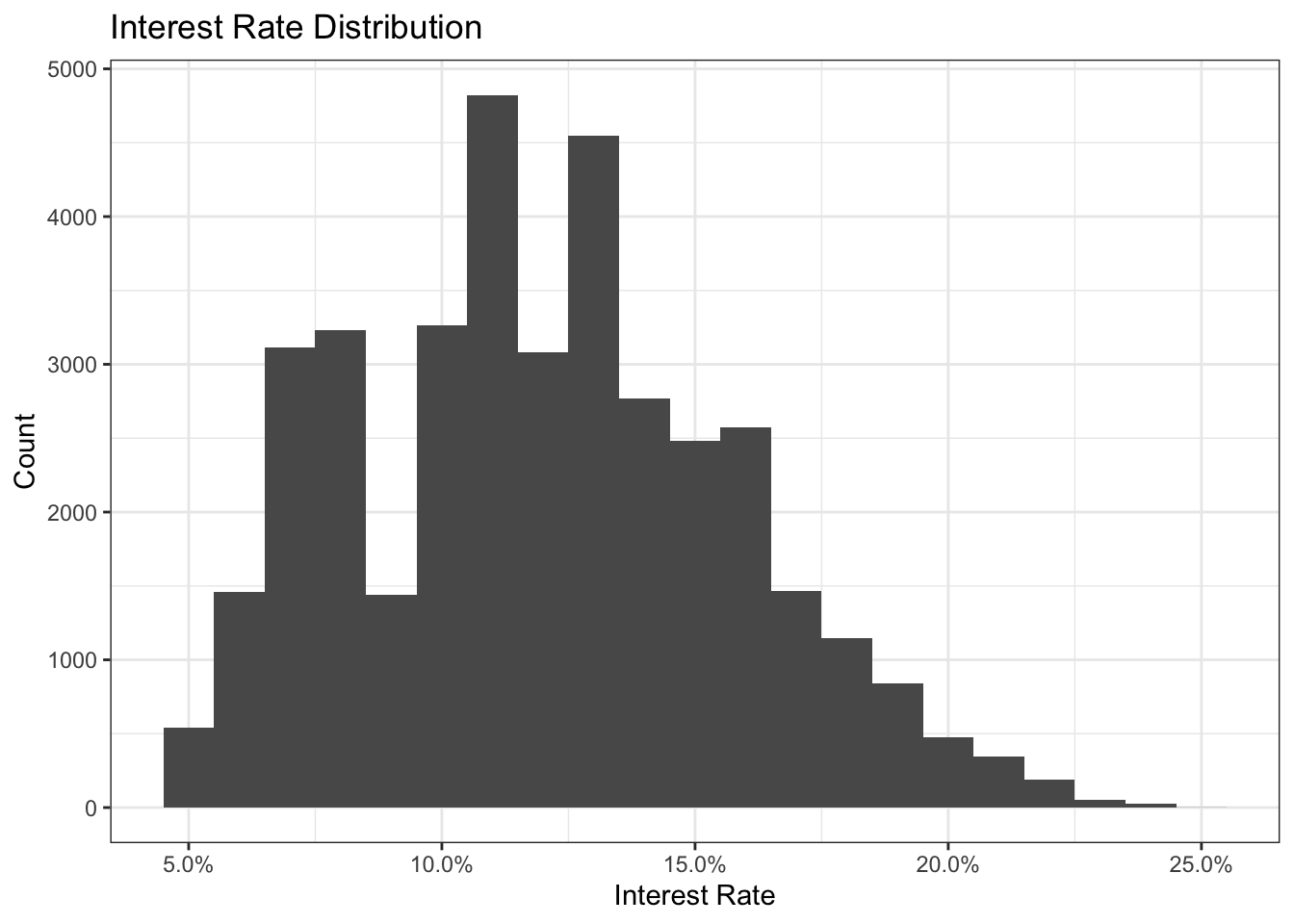
The histogram seems to be fairly normally distributed. There seem to be gaps in frequency of certain interest rates (so not the usual smooth,continuous looking function we would hope for) but this could be due to fixed ranges of interest rates that are charged. The mode is around 11%.
# Histogram of interest rates, different colours per term (36 or 60)
ggplot(lc_clean, aes(x=int_rate, fill=term))+
  geom_histogram(binwidth = 0.01)+
  theme_bw()+
  scale_x_continuous(labels=scales::percent)+
  labs(
    title = "Loan for 36 or 60 months?",
    x= "Interest Rate",
    y="Count",
    fill = "Loan term (months)"
  )+
  NULL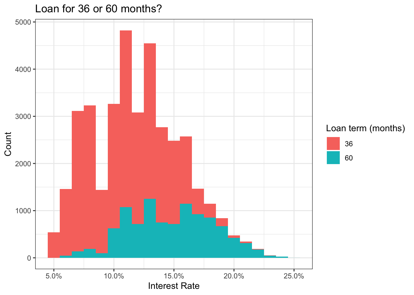
This graph reveals that there are generally more 36-months loans than 60-months loans. Higher and lower interest rates are spread relatively evenly between the two although only very few 60-months loans have an interest rate below 10%.
# Histogram of interest rates but use different color for loans of different grades
ggplot(lc_clean, aes(x=int_rate, fill=grade))+
  geom_histogram(binwidth = 0.01)+
 theme_bw()+
   scale_x_continuous(labels=scales::percent)+
  labs(
    title = "Higher grade, lower interest",
    x= "Interest Rate",
    y="Count",
    fill = "Grade"
  )+
  NULL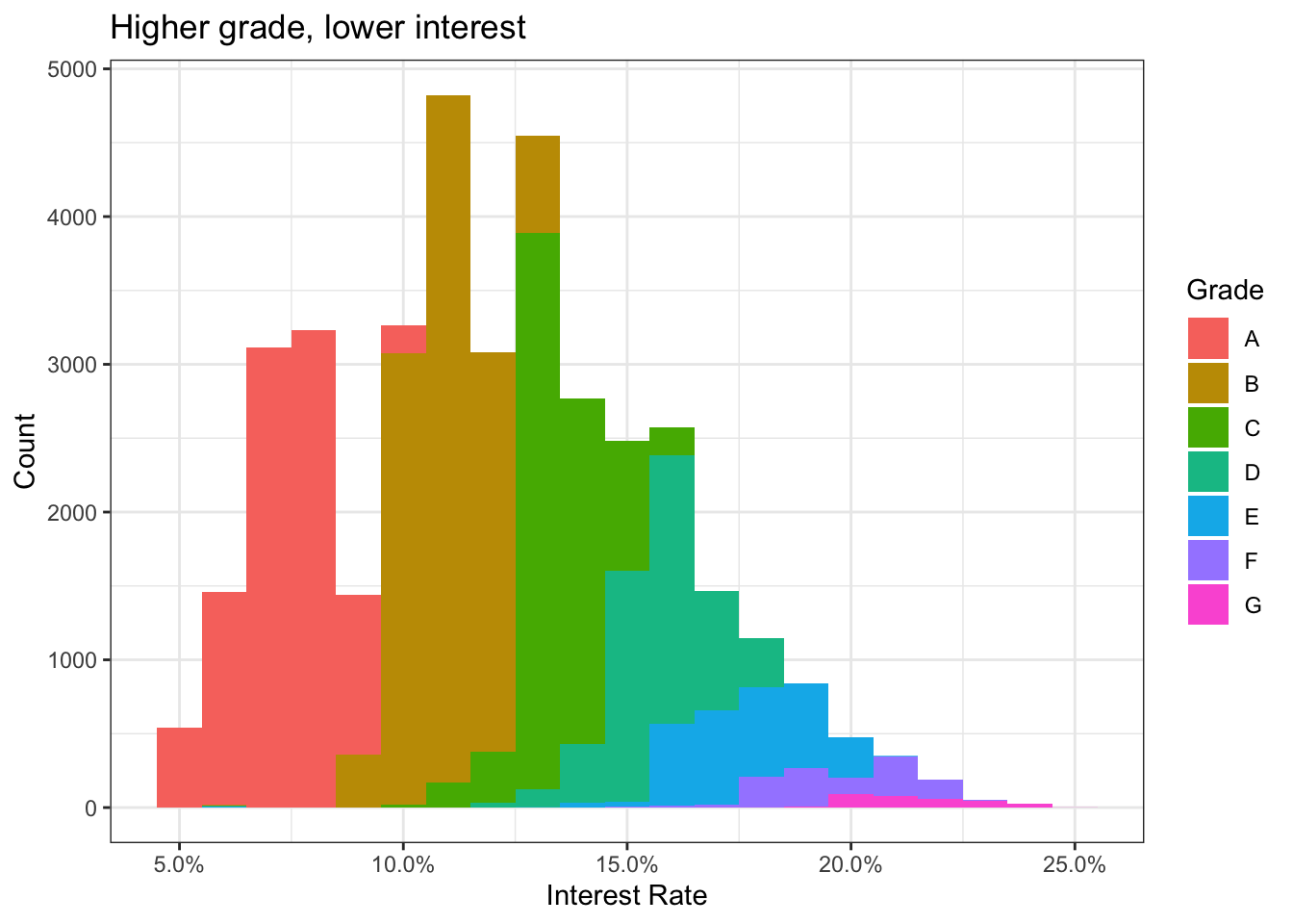
# Density plot with colour for different grades.
ggplot(lc_clean, aes(x=int_rate, fill=grade, alpha = 0.2))+
  geom_density()+
  facet_grid(rows = vars(grade))+
  theme_bw()+
  theme(legend.position = "none")+
  scale_x_continuous(labels = scales::percent)+
  labs(title = "Higher grade, lower interest 2.0",
       x="Interest Rate",
       y = "Density")+
  NULL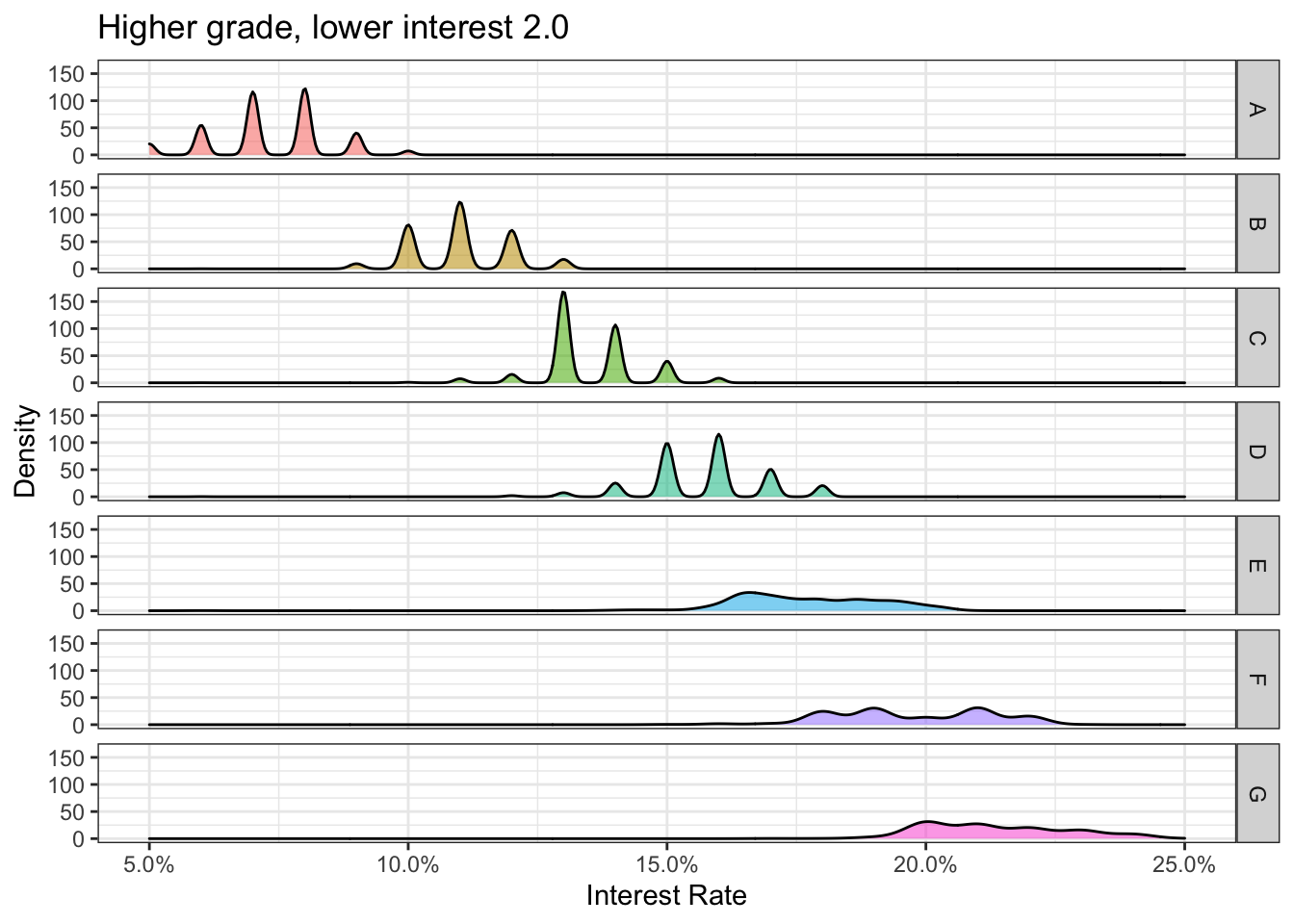
The histogram and the density plot above reveal insights into the division of interest rates by grade rating. The lending club seems to give out mostly grade A, B and C loans. There seems to be a negative relationship between grade rating and interest rates where the higher the grade, the lower the interest charged.
# Scatter plot of loan amount against interest rate and with  the line of best fit
ggplot(lc_clean, aes(x=loan_amnt, y=int_rate))+
  geom_point(size = 0.1, alpha = 0.5)+
  geom_smooth(method="lm", se = 0)+
  theme_bw()+
  scale_y_continuous(labels=scales::percent)+
  scale_x_continuous(labels=scales::dollar_format())+
  labs(
    title = "More money, higher interest ",
    x= "Loan Amount",
    y="Interest Rate"
  )+
  NULL
## `geom_smooth()` using formula 'y ~ x'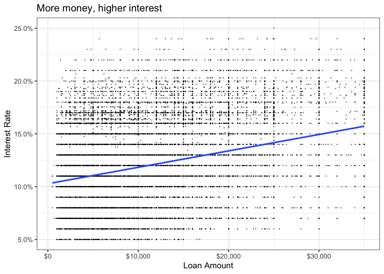
We can see a positive correlation between loan amount and interest rate, indicating, the higher the loan amount, the higher the interest rate.
# Produce a scatter plot of annual income against interest rate and add visually the line of best fit
ggplot(lc_clean, aes(x=annual_inc, y=int_rate))+
  geom_point(size = 0.1, alpha = 0.5)+
  geom_smooth(method="lm", se = 0)+
  theme_bw()+
  scale_y_continuous(labels=scales::percent)+
  #reduce scale to see stronger result (sacrificed 1 data point)
  scale_x_continuous(labels=scales::dollar_format(),limits=c(0,2100000))+
  labs(
    title = "Earn more, pay more",
    x= "Annual Income", y="Interest Rate")+
  NULL
## `geom_smooth()` using formula 'y ~ x'## Warning: Removed 1 rows containing non-finite values (stat_smooth).## Warning: Removed 1 rows containing missing values (geom_point).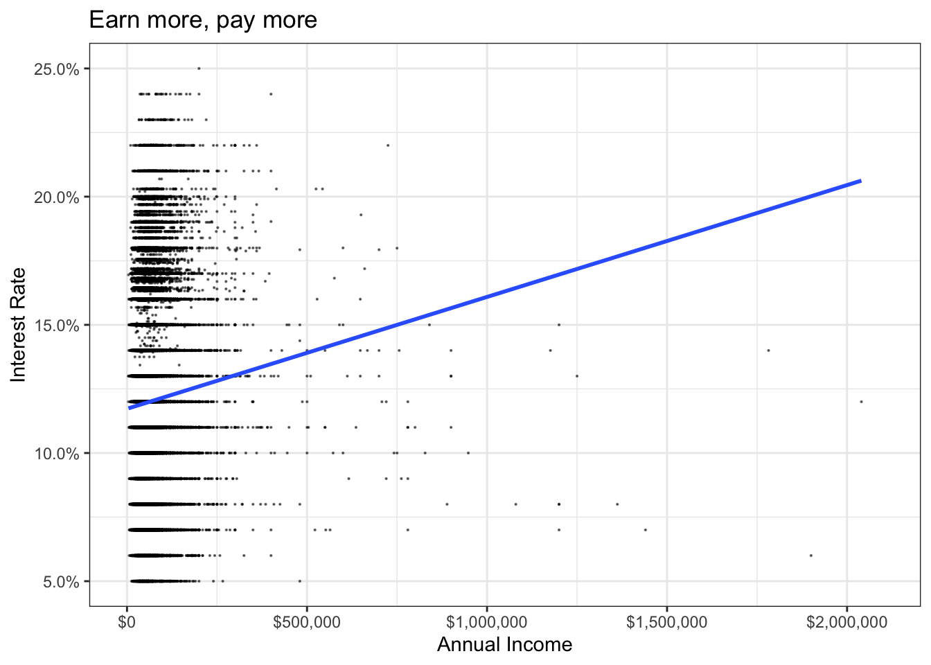
The graph seems to reflect a positive correlation between income and interest rate, indicating, the higher the income, the higher the interest rate to pay for a loan.
# In the same axes, produce box plots of the interest rate for every value of delinquencies
ggplot(lc_clean, aes(x=delinq_2yrs, y=int_rate, color=delinq_2yrs))+
  geom_boxplot()+
  theme_bw()+
  scale_y_continuous(labels=scales::percent)+
  theme(legend.position = "none")+
  labs(
    title = "Do delinquencies in the last two years have an effect \non interest rate charged?",
    x= "Number of delinquecies in last two years", y="Interest Rate"
  )+
  NULL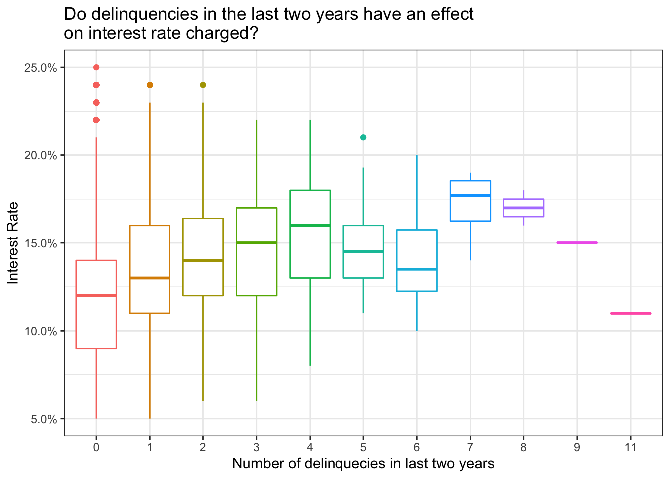
There seems to be a positive correlation between interest rates and loans with 0-4 delinquencies in 2 years. However, there seems to be an inverse correlation from 4-6. There are few loan observations with 7-8 delinquencies and even fewer observations of over 8 delinquencies which makes the interpretation more difficult. This analysis may benefit from re-categorizing.
#boxplot with colour for different home_ownerhsip
lc_clean$home_ownership <- factor(lc_clean$home_ownership, levels = c("RENT", "OTHER", "MORTGAGE", "OWN", "NONE"))

ggplot(lc_clean, aes(x=home_ownership, y=int_rate, colour=home_ownership))+
  geom_boxplot()+
  theme_bw()+
  theme(legend.position = "none")+
  scale_y_continuous(labels=scales::percent)+
  labs(title = "Does Home Ownership have an influence on interest rate charged?",
    y="Interest Rate",
    x="Home Ownership")+
  NULL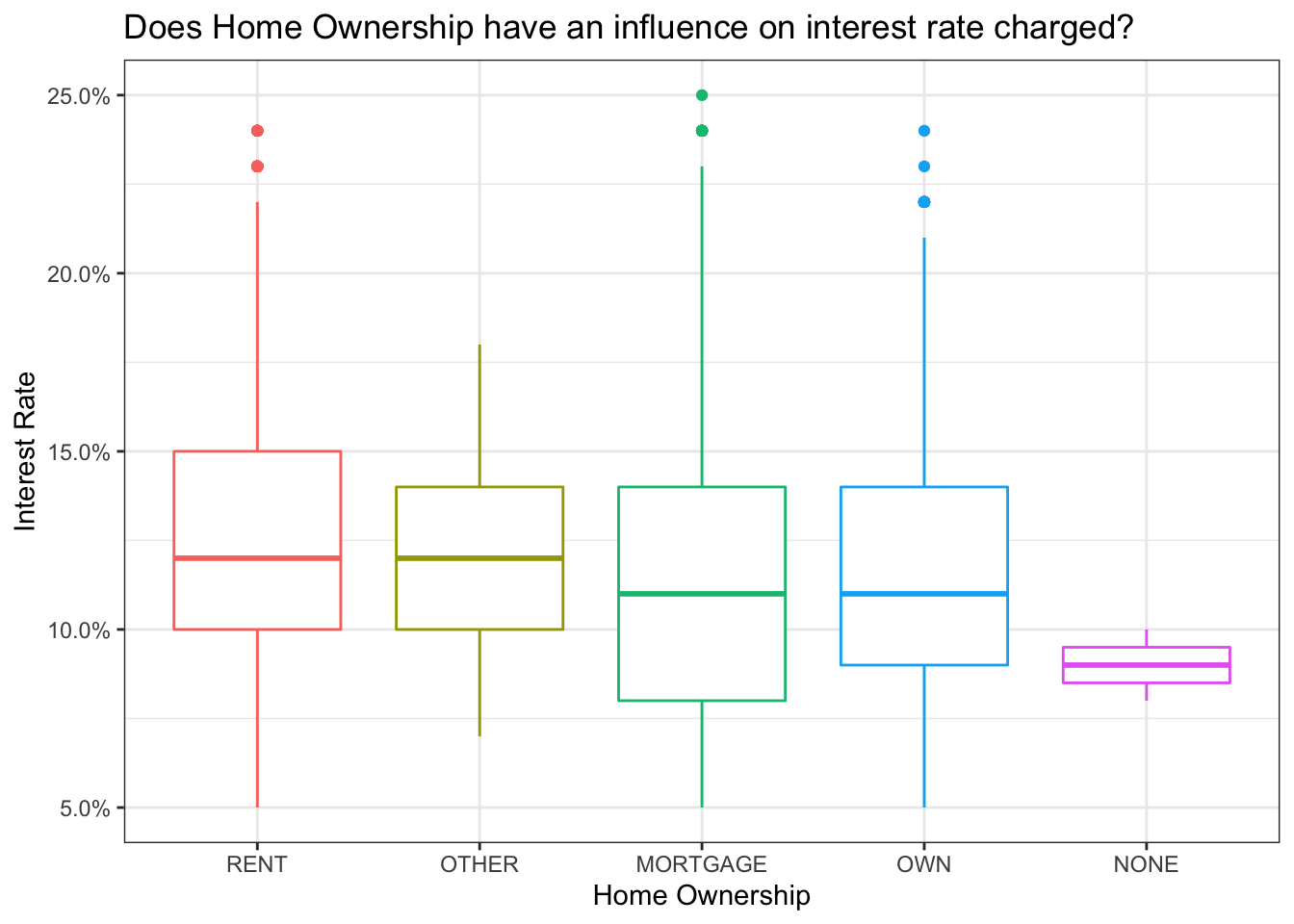
We cannot find a clear relationship of the influence of the kind of home ownership the people taking on a loan have with the interest rates they will be charged.
Scatterplot- Correlation Matrix
We build a correlation table for the numerical variables and investigate the impact of a number of variables on the interest rate charged graphically
# correlation table using GGally::ggpairs()
# this takes a while to plot
lc_clean %>%
  select(term, loan_amnt, dti,annual_inc, int_rate) %>% #keep Y variable last
  ggpairs(aes(alpha = 0.2, colour = term)) +
  theme_bw()
## `stat_bin()` using `bins = 30`. Pick better value with `binwidth`.
## `stat_bin()` using `bins = 30`. Pick better value with `binwidth`.
## `stat_bin()` using `bins = 30`. Pick better value with `binwidth`.
## `stat_bin()` using `bins = 30`. Pick better value with `binwidth`.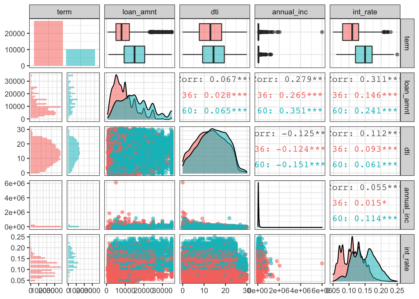
Estimate simple linear regression models
We start with a simple but quite powerful model.
#Use the lm command to estimate a regression model with the following variables "loan_amnt",  "term", "dti", "annual_inc", and "grade"

model1<-lm( int_rate~loan_amnt+term+dti+annual_inc+grade, data=lc_clean)

summary(model1)
##
## Call:
## lm(formula = int_rate ~ loan_amnt + term + dti + annual_inc +
## grade, data = lc_clean)
##
## Residuals:
## Min 1Q Median 3Q Max
## -0.118827 -0.007035 -0.000342 0.006828 0.035081
##
## Coefficients:
## Estimate Std. Error t value Pr(>|t|)
## (Intercept) 7.169e-02 1.689e-04 424.363 < 2e-16 ***
## loan_amnt 1.475e-07 8.284e-09 17.809 < 2e-16 ***
## term60 3.608e-03 1.419e-04 25.431 < 2e-16 ***
## dti 4.328e-05 8.269e-06 5.234 1.66e-07 ***
## annual_inc -9.734e-10 9.283e-10 -1.049 0.294
## gradeB 3.554e-02 1.492e-04 238.248 < 2e-16 ***
## gradeC 6.016e-02 1.658e-04 362.783 < 2e-16 ***
## gradeD 8.172e-02 1.906e-04 428.746 < 2e-16 ***
## gradeE 9.999e-02 2.483e-04 402.660 < 2e-16 ***
## gradeF 1.195e-01 3.673e-04 325.408 < 2e-16 ***
## gradeG 1.355e-01 6.208e-04 218.245 < 2e-16 ***
## ---
## Signif. codes: 0 '***' 0.001 '**' 0.01 '*' 0.05 '.' 0.1 ' ' 1
##
## Residual standard error: 0.01056 on 37858 degrees of freedom
## Multiple R-squared: 0.9198, Adjusted R-squared: 0.9197
## F-statistic: 4.34e+04 on 10 and 37858 DF, p-value: < 2.2e-16ncvTest(model1) # check inferential capabilities of this model/heteroskedasticity## Non-constant Variance Score Test
## Variance formula: ~ fitted.values
## Chisquare = 240.3426, Df = 1, p = < 2.22e-16vif(model1) # check inferential capabilities of this model/multicolinearity## GVIF Df GVIF^(1/(2*Df))
## loan_amnt 1.298936 1 1.139709
## term 1.345672 1 1.160031
## dti 1.038820 1 1.019225
## annual_inc 1.113410 1 1.055183
## grade 1.303314 6 1.022321crPlots(model1)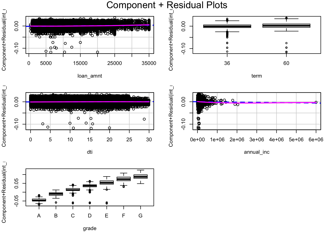
Q2. Questions on model 1
- Are all variables statistically significant?
- How do we interpret the coefficient of the Term60 dummy variable? Of the grade B dummy variable?
- How much explanatory power does the model have?
- Approximately, how wide would the 95% confidence interval of any prediction based on this model be?
- Yes, all explanatory variables, except annual_income, are statistically significant because the t-value >> |2| (Using 2 as a 5% benchmark).
- The model assumes a baseline term of 36 months, The term60 coefficient is added to the interest rate estimate if the underlying loan has a term structure of 60 months. The coefficient of term60 is 3.608e-03, this implies that compared to a 36 month loan, the interest rate of a 60 month loan will be on average 0.36% higher. The model further assumes a baseline grade A quality. The coefficient of grade B loans is 3.554e-02, which implies that compared to a grade A loan, the interest rate of a grade B loan will be 3.55% higher.
- The model captures/explains 91.97% of the variability of interest rates, as shown by the adjusted R-squared.
- The 95% confidence interval for any prediction will be (+/- 2*RSE). With an RSE of 0.01056, the 95% confidence interval is (-2.112, 2.112), meaning a prediction width of 4.224%.
Feature Engineering
Let’s build progressively more complex models with more features.
#Add to the previous model an interaction between loan amount and grade. Use the "var1*var2" notation to define an interaction term in the linear regression model. This will add the interaction and the individual variables to the model.

model2 <-lm(int_rate ~ loan_amnt + term+dti + annual_inc + grade + loan_amnt*grade, data=lc_clean)
summary(model2)
##
## Call:
## lm(formula = int_rate ~ loan_amnt + term + dti + annual_inc +
## grade + loan_amnt * grade, data = lc_clean)
##
## Residuals:
## Min 1Q Median 3Q Max
## -0.119807 -0.007230 -0.000057 0.006588 0.037460
##
## Coefficients:
## Estimate Std. Error t value Pr(>|t|)
## (Intercept) 7.171e-02 2.345e-04 305.762 < 2e-16 ***
## loan_amnt 1.528e-07 2.028e-08 7.537 4.91e-14 ***
## term60 3.793e-03 1.424e-04 26.636 < 2e-16 ***
## dti 3.836e-05 8.250e-06 4.649 3.34e-06 ***
## annual_inc -1.224e-09 9.249e-10 -1.324 0.18564
## gradeB 3.623e-02 2.732e-04 132.619 < 2e-16 ***
## gradeC 6.198e-02 2.988e-04 207.452 < 2e-16 ***
## gradeD 8.082e-02 3.483e-04 232.034 < 2e-16 ***
## gradeE 9.633e-02 4.625e-04 208.293 < 2e-16 ***
## gradeF 1.143e-01 7.735e-04 147.699 < 2e-16 ***
## gradeG 1.327e-01 1.551e-03 85.580 < 2e-16 ***
## loan_amnt:gradeB -6.617e-08 2.441e-08 -2.710 0.00673 **
## loan_amnt:gradeC -1.704e-07 2.621e-08 -6.500 8.14e-11 ***
## loan_amnt:gradeD 6.703e-08 2.798e-08 2.395 0.01662 *
## loan_amnt:gradeE 2.209e-07 3.016e-08 7.323 2.47e-13 ***
## loan_amnt:gradeF 2.779e-07 4.136e-08 6.720 1.85e-11 ***
## loan_amnt:gradeG 1.265e-07 7.260e-08 1.743 0.08140 .
## ---
## Signif. codes: 0 '***' 0.001 '**' 0.01 '*' 0.05 '.' 0.1 ' ' 1
##
## Residual standard error: 0.01052 on 37852 degrees of freedom
## Multiple R-squared: 0.9204, Adjusted R-squared: 0.9204
## F-statistic: 2.735e+04 on 16 and 37852 DF, p-value: < 2.2e-16#Add to the model the square and the cube of annual income. Use the poly(var_name,3) command as a variable in the linear regression model.
model3 <- lm(int_rate ~ loan_amnt + term + dti + grade + loan_amnt*grade + poly(annual_inc,3), data=lc_clean)
summary(model3)##
## Call:
## lm(formula = int_rate ~ loan_amnt + term + dti + grade + loan_amnt *
## grade + poly(annual_inc, 3), data = lc_clean)
##
## Residuals:
## Min 1Q Median 3Q Max
## -0.119814 -0.007238 -0.000065 0.006594 0.037471
##
## Coefficients:
## Estimate Std. Error t value Pr(>|t|)
## (Intercept) 7.161e-02 2.279e-04 314.200 < 2e-16 ***
## loan_amnt 1.556e-07 2.047e-08 7.600 3.03e-14 ***
## term60 3.786e-03 1.426e-04 26.546 < 2e-16 ***
## dti 3.761e-05 8.294e-06 4.535 5.79e-06 ***
## gradeB 3.623e-02 2.732e-04 132.611 < 2e-16 ***
## gradeC 6.198e-02 2.988e-04 207.398 < 2e-16 ***
## gradeD 8.081e-02 3.483e-04 231.999 < 2e-16 ***
## gradeE 9.633e-02 4.625e-04 208.283 < 2e-16 ***
## gradeF 1.143e-01 7.736e-04 147.695 < 2e-16 ***
## gradeG 1.327e-01 1.551e-03 85.573 < 2e-16 ***
## poly(annual_inc, 3)1 -1.589e-02 1.117e-02 -1.423 0.1549
## poly(annual_inc, 3)2 6.296e-03 1.086e-02 0.580 0.5621
## poly(annual_inc, 3)3 -8.981e-03 1.084e-02 -0.828 0.4076
## loan_amnt:gradeB -6.633e-08 2.442e-08 -2.717 0.0066 **
## loan_amnt:gradeC -1.703e-07 2.621e-08 -6.498 8.23e-11 ***
## loan_amnt:gradeD 6.709e-08 2.798e-08 2.398 0.0165 *
## loan_amnt:gradeE 2.209e-07 3.016e-08 7.324 2.45e-13 ***
## loan_amnt:gradeF 2.780e-07 4.136e-08 6.722 1.82e-11 ***
## loan_amnt:gradeG 1.270e-07 7.260e-08 1.750 0.0801 .
## ---
## Signif. codes: 0 '***' 0.001 '**' 0.01 '*' 0.05 '.' 0.1 ' ' 1
##
## Residual standard error: 0.01052 on 37850 degrees of freedom
## Multiple R-squared: 0.9204, Adjusted R-squared: 0.9204
## F-statistic: 2.431e+04 on 18 and 37850 DF, p-value: < 2.2e-16#Continuing with the previous model, instead of annual income as a continuous variable break it down into quartiles and use quartile dummy variables.
lc_clean <- lc_clean %>%
mutate(quartiles_annual_inc = as.factor(ntile(annual_inc, 4)))
model4 <-lm(int_rate ~ loan_amnt + term + dti + grade + loan_amnt*grade + quartiles_annual_inc, data=lc_clean)
summary(model4) ##
## Call:
## lm(formula = int_rate ~ loan_amnt + term + dti + grade + loan_amnt *
## grade + quartiles_annual_inc, data = lc_clean)
##
## Residuals:
## Min 1Q Median 3Q Max
## -0.119767 -0.007203 -0.000064 0.006596 0.037581
##
## Coefficients:
## Estimate Std. Error t value Pr(>|t|)
## (Intercept) 7.187e-02 2.414e-04 297.700 < 2e-16 ***
## loan_amnt 1.615e-07 2.048e-08 7.889 3.13e-15 ***
## term60 3.781e-03 1.425e-04 26.532 < 2e-16 ***
## dti 3.672e-05 8.259e-06 4.446 8.78e-06 ***
## gradeB 3.622e-02 2.733e-04 132.524 < 2e-16 ***
## gradeC 6.196e-02 2.989e-04 207.272 < 2e-16 ***
## gradeD 8.079e-02 3.484e-04 231.877 < 2e-16 ***
## gradeE 9.632e-02 4.625e-04 208.273 < 2e-16 ***
## gradeF 1.143e-01 7.735e-04 147.723 < 2e-16 ***
## gradeG 1.327e-01 1.551e-03 85.570 < 2e-16 ***
## quartiles_annual_inc2 -2.619e-04 1.548e-04 -1.692 0.09068 .
## quartiles_annual_inc3 -3.992e-04 1.590e-04 -2.510 0.01208 *
## quartiles_annual_inc4 -5.382e-04 1.692e-04 -3.181 0.00147 **
## loan_amnt:gradeB -6.638e-08 2.441e-08 -2.719 0.00655 **
## loan_amnt:gradeC -1.699e-07 2.621e-08 -6.483 9.10e-11 ***
## loan_amnt:gradeD 6.770e-08 2.798e-08 2.419 0.01555 *
## loan_amnt:gradeE 2.203e-07 3.016e-08 7.304 2.85e-13 ***
## loan_amnt:gradeF 2.766e-07 4.136e-08 6.687 2.30e-11 ***
## loan_amnt:gradeG 1.267e-07 7.259e-08 1.746 0.08089 .
## ---
## Signif. codes: 0 '***' 0.001 '**' 0.01 '*' 0.05 '.' 0.1 ' ' 1
##
## Residual standard error: 0.01052 on 37850 degrees of freedom
## Multiple R-squared: 0.9204, Adjusted R-squared: 0.9204
## F-statistic: 2.432e+04 on 18 and 37850 DF, p-value: < 2.2e-16#Compare the performance of these four models using the anova command
anova(model1, model2, model3, model4)| Res.Df | RSS | Df | Sum of Sq | F | Pr(>F) |
|---|---|---|---|---|---|
| 3.79e+04 | 4.22 | ||||
| 3.79e+04 | 4.19 | 6 | 0.0332 | 50 | 1.64e-61 |
| 3.78e+04 | 4.19 | 2 | 0.000107 | 0.484 | 0.616 |
| 3.78e+04 | 4.19 | 0 | 0.000915 |
#Presentation of all results
huxreg(model1, model2, model3, model4)| (1) | (2) | (3) | (4) | |
|---|---|---|---|---|
| (Intercept) | 0.072 *** | 0.072 *** | 0.072 *** | 0.072 *** |
| (0.000) | (0.000) | (0.000) | (0.000) | |
| loan_amnt | 0.000 *** | 0.000 *** | 0.000 *** | 0.000 *** |
| (0.000) | (0.000) | (0.000) | (0.000) | |
| term60 | 0.004 *** | 0.004 *** | 0.004 *** | 0.004 *** |
| (0.000) | (0.000) | (0.000) | (0.000) | |
| dti | 0.000 *** | 0.000 *** | 0.000 *** | 0.000 *** |
| (0.000) | (0.000) | (0.000) | (0.000) | |
| annual_inc | -0.000 | -0.000 | ||
| (0.000) | (0.000) | |||
| gradeB | 0.036 *** | 0.036 *** | 0.036 *** | 0.036 *** |
| (0.000) | (0.000) | (0.000) | (0.000) | |
| gradeC | 0.060 *** | 0.062 *** | 0.062 *** | 0.062 *** |
| (0.000) | (0.000) | (0.000) | (0.000) | |
| gradeD | 0.082 *** | 0.081 *** | 0.081 *** | 0.081 *** |
| (0.000) | (0.000) | (0.000) | (0.000) | |
| gradeE | 0.100 *** | 0.096 *** | 0.096 *** | 0.096 *** |
| (0.000) | (0.000) | (0.000) | (0.000) | |
| gradeF | 0.120 *** | 0.114 *** | 0.114 *** | 0.114 *** |
| (0.000) | (0.001) | (0.001) | (0.001) | |
| gradeG | 0.135 *** | 0.133 *** | 0.133 *** | 0.133 *** |
| (0.001) | (0.002) | (0.002) | (0.002) | |
| loan_amnt:gradeB | -0.000 ** | -0.000 ** | -0.000 ** | |
| (0.000) | (0.000) | (0.000) | ||
| loan_amnt:gradeC | -0.000 *** | -0.000 *** | -0.000 *** | |
| (0.000) | (0.000) | (0.000) | ||
| loan_amnt:gradeD | 0.000 * | 0.000 * | 0.000 * | |
| (0.000) | (0.000) | (0.000) | ||
| loan_amnt:gradeE | 0.000 *** | 0.000 *** | 0.000 *** | |
| (0.000) | (0.000) | (0.000) | ||
| loan_amnt:gradeF | 0.000 *** | 0.000 *** | 0.000 *** | |
| (0.000) | (0.000) | (0.000) | ||
| loan_amnt:gradeG | 0.000 | 0.000 | 0.000 | |
| (0.000) | (0.000) | (0.000) | ||
| poly(annual_inc, 3)1 | -0.016 | |||
| (0.011) | ||||
| poly(annual_inc, 3)2 | 0.006 | |||
| (0.011) | ||||
| poly(annual_inc, 3)3 | -0.009 | |||
| (0.011) | ||||
| quartiles_annual_inc2 | -0.000 | |||
| (0.000) | ||||
| quartiles_annual_inc3 | -0.000 * | |||
| (0.000) | ||||
| quartiles_annual_inc4 | -0.001 ** | |||
| (0.000) | ||||
| N | 37869 | 37869 | 37869 | 37869 |
| R2 | 0.920 | 0.920 | 0.920 | 0.920 |
| logLik | 118612.653 | 118762.008 | 118762.492 | 118766.633 |
| AIC | -237201.305 | -237488.016 | -237484.984 | -237493.266 |
| *** p < 0.001; ** p < 0.01; * p < 0.05. | ||||
Q3. Questions on models 1-4
- Which of the four models has the most explanatory power in sample?
- In model 2, how do we interpret the estimated coefficient of the interaction term between grade B and loan amount?
- The problem of multicolinearity describes the situations where one feature is highly correlated with other features (or with a linear combination of other features). If our goal is to use the model to make predictions, should we be concerned by the problem of multicolinearity? Why, or why not?
- The adjusted R-Squareds of all 4 models are all approx. at 92% explained variance and very very similar. Model 2, 3 and 4 have the same, highest adjusted R-squared of 0.9204. Nevertheless, the lowest adjusted R-squared among the models is 0.9197 (model1). The difference is rather insignificant. Considering the RSS, we find that model 4 has the lowest RSS at 4.1850. Model 2 and 3’s RSS are very similar while also model1’s RSS of 4.2192 is not significantly larger. Strictly comparing numbres, model4 has the highest explanatory power. However, as there are no signficiant differences in explanatory power between the four models, for simiplicity of understanding (less complex) and because it is still a very powerful statistical model with 91.97% explanatory power, model1 is preferable. We also note that model1 has no multiocolinearity issues which would mean this model could be usued for causal inference. However, after running a Breusch-Pagan test, we reject the null and find evidence of heteroskedasticity which affects the causal inferential capabilities of the model but not its predictive power.
- The coefficient of the interaction term loan amount:gradeB is -6.617e-08. This implies that on average (1.528e-07 - 6.617e-08 = 8.663e-08) an additional $100K of loan will increase the interest rate of a grade B loan by 0.8663%.
- For the purpose of prediction multicolinearity is not an issue, unlike in inference. This is because multicolinearity can cause issues in the Standard Error of the coeffiencients and coefficients estimates values, however removing multicolinearity does not alter the predictive power/capacity of the overall model, both models(with and without multicolinearity issues) will produce identical results for fitted values and prediction intervals.
Out of sample testing
Checking the predictive accuracy of model2 by holding out a subset of the data to use as testing. This method is sometimes referred to as the hold-out method for out-of-sample testing.
#split the data in dataframe called "testing" and another one called  "training". The "training" dataframe should have 80% of the data and the "testing" dataframe 20%.

set.seed(1456)
train_test_split <- initial_split(lc_clean, prop = 0.8)
training <- training(train_test_split)
testing <- testing(train_test_split)


#Fit model2 on the training set
model2_training<-lm(int_rate ~ loan_amnt + term+ dti + annual_inc + grade +grade:loan_amnt, training)


#Calculate the RMSE of the model in the training set (in sample)
rmse_training<-sqrt(mean((residuals(model2_training))^2))
#USe the model to make predictions out of sample in the testing set
pred<-predict(model2_training,testing)
#Calculate the RMSE of the model in the testing set (out of sample)
rmse_testing<- RMSE(pred,testing$int_rate)


data.frame(RMSE_Training=rmse_training,RMSE_Testing=rmse_testing)| RMSE_Training | RMSE_Testing |
|---|---|
| 0.0105 | 0.0105 |
rmse_training # = 0.01053025 (in-sample)## [1] 0.01053025rmse_testing # = 0.01045298 (out-of-sample)## [1] 0.01045298(rmse_testing/rmse_training-1) # = -0.007338007## [1] -0.007338007Q4. Question on hold-out-method model
How much does the predictive accuracy of model 2 deteriorate when we move from in sample to out of sample testing? Is this sensitive to the random seed chosen? Is there any evidence of overfitting?
The predictive accuracy of the model does not deteriorate since the RMSE decreases by approx. 0.7% from 0.01053025 to 0.01045298 from the training to the testing set respectively. As the RMSE measures the error of our model in predicting data, we see that the smaller RMSE means that the predictive accuracy increases as we move from in sample to out of sample testing. The difference in RMSEs is, however very small, which implies that the model has a good fit in genral across both the training and testing data, again implying that it has good predictive capacity. Nevertheless, we cannot rule out that, with a different seed set, the RMSE may not be decresasing from in- to out-of-sample testing.
This method/model is sensitive to the random seed chosen as setting a different seed, changes the resulting values slightly. Setting a seed helps with reproducing the model. However, fixing the training and testing data can create differences in the predictive capacity of the model as the random allocation of data points into a training and testing set can skew the model’s predictive accuracy if the training and testing data are not well diversified enough.
If the RMSE of the testing set is very different from that of the training set, this would be an indication of overfitting the data. The RMSE of the testing set is only 0.7% smaller than that of the training set; assuming a threshold of 10% (minimial difference at which we would conclude overfitting), we find no signs of overfitting.
k-fold cross validation
We can also do out of sample testing using the method of k-fold cross validation. Using the caret package this is easy.
#the method "cv" stands for cross validation. We re going to create 10 folds.

control <- trainControl (
    method="cv",
    number=10,
    verboseIter=TRUE) #by setting this to true the model will report its progress after each estimation

#we are going to train the model and report the results using k-fold cross validation
plsFit<-train(
    int_rate ~ loan_amnt + term+ dti + annual_inc + grade +grade:loan_amnt ,
    lc_clean,
   method = "lm",
    trControl = control
   )
## + Fold01: intercept=TRUE
## - Fold01: intercept=TRUE
## + Fold02: intercept=TRUE
## - Fold02: intercept=TRUE
## + Fold03: intercept=TRUE
## - Fold03: intercept=TRUE
## + Fold04: intercept=TRUE
## - Fold04: intercept=TRUE
## + Fold05: intercept=TRUE
## - Fold05: intercept=TRUE
## + Fold06: intercept=TRUE
## - Fold06: intercept=TRUE
## + Fold07: intercept=TRUE
## - Fold07: intercept=TRUE
## + Fold08: intercept=TRUE
## - Fold08: intercept=TRUE
## + Fold09: intercept=TRUE
## - Fold09: intercept=TRUE
## + Fold10: intercept=TRUE
## - Fold10: intercept=TRUE
## Aggregating results
## Fitting final model on full training setsummary(plsFit)##
## Call:
## lm(formula = .outcome ~ ., data = dat)
##
## Residuals:
## Min 1Q Median 3Q Max
## -0.119807 -0.007230 -0.000057 0.006588 0.037460
##
## Coefficients:
## Estimate Std. Error t value Pr(>|t|)
## (Intercept) 7.171e-02 2.345e-04 305.762 < 2e-16 ***
## loan_amnt 1.528e-07 2.028e-08 7.537 4.91e-14 ***
## term60 3.793e-03 1.424e-04 26.636 < 2e-16 ***
## dti 3.836e-05 8.250e-06 4.649 3.34e-06 ***
## annual_inc -1.224e-09 9.249e-10 -1.324 0.18564
## gradeB 3.623e-02 2.732e-04 132.619 < 2e-16 ***
## gradeC 6.198e-02 2.988e-04 207.452 < 2e-16 ***
## gradeD 8.082e-02 3.483e-04 232.034 < 2e-16 ***
## gradeE 9.633e-02 4.625e-04 208.293 < 2e-16 ***
## gradeF 1.143e-01 7.735e-04 147.699 < 2e-16 ***
## gradeG 1.327e-01 1.551e-03 85.580 < 2e-16 ***
## `loan_amnt:gradeB` -6.617e-08 2.441e-08 -2.710 0.00673 **
## `loan_amnt:gradeC` -1.704e-07 2.621e-08 -6.500 8.14e-11 ***
## `loan_amnt:gradeD` 6.703e-08 2.798e-08 2.395 0.01662 *
## `loan_amnt:gradeE` 2.209e-07 3.016e-08 7.323 2.47e-13 ***
## `loan_amnt:gradeF` 2.779e-07 4.136e-08 6.720 1.85e-11 ***
## `loan_amnt:gradeG` 1.265e-07 7.260e-08 1.743 0.08140 .
## ---
## Signif. codes: 0 '***' 0.001 '**' 0.01 '*' 0.05 '.' 0.1 ' ' 1
##
## Residual standard error: 0.01052 on 37852 degrees of freedom
## Multiple R-squared: 0.9204, Adjusted R-squared: 0.9204
## F-statistic: 2.735e+04 on 16 and 37852 DF, p-value: < 2.2e-16Q5. Question on k-fold method model
Compare the out-of-sample RMSE of 10-fold cross validation and the hold-out method. Are they different? Which do we think is more reliable? Are there any drawbacks to the k-fold cross validation method compared to the hold-out method?
The out-of sample (testing set) RMSE of the hold-out method is 0.01045298 while the 10-fold cross validation method yields an RMSE of 0.01052. These values do not differ very significantly as the k-fold RMSE is approx. 0.6% greater than the hold-out RMSE.
While the simplest way for cross validation is the hold-out method, the k-fold cross validation method is a way to improve it. In the k-fold method, each data point will be included in a testing set once and will be included k-1 times in the training set. This is beneficial as it is less relevant how the data is divided. Additionally, with increasing k, we reduce the estimated coefficient’s variance. A drawback of the k-fold cross validation compared to the hold out method is that the k-fold method takes k times, here 10 times (as we used 10 folds/k = 10), as much computation to reach a result as its training alogrithm has to be rerun from the very beginning k times (here, 10 times).
Sample size estimation and learning curves
We can use the hold out method for out-of-sample testing to check if we have a sufficiently large sample to estimate the model reliably. The idea is to set aside some of the data as a testing set. From the remaining data draw progressively larger training sets and check how the performance of the model on the testing set changes. If the performance no longer improves with larger datasets we know we have a large enough sample. The code below does this. Examine it and run it with different random seeds.
#select a testing dataset (25% of all data)
set.seed(12)

train_test_split <- initial_split(lc_clean, prop = 0.75)
remaining <- training(train_test_split)
testing <- testing(train_test_split)

#We are now going to run 30 models starting from a tiny training set drawn from the training data and progressively increasing its size. The testing set remains the same in all iterations.

#initiating the model by setting some parameters to zero
rmse_sample <- 0
sample_size<-0
Rsq_sample<-0

for(i in 1:30) {
#from the remaining dataset select a smaller subset to training the data
set.seed(100)
sample

  learning_split <- initial_split(remaining, prop = i/200)
  training <- training(learning_split)
  sample_size[i]=nrow(training)

  #traing the model on the small dataset
  model3<-lm(int_rate ~ loan_amnt + term+ dti + annual_inc + grade + grade:loan_amnt, training)
  #test the performance of the model on the large testing dataset. This stays fixed for all iterations.
  pred<-predict(model3,testing)
  rmse_sample[i]<-RMSE(pred,testing$int_rate)
  Rsq_sample[i]<-R2(pred,testing$int_rate)
}
## Warning in predict.lm(model3, testing): prediction from a rank-deficient fit may
## be misleadingplot(sample_size,rmse_sample)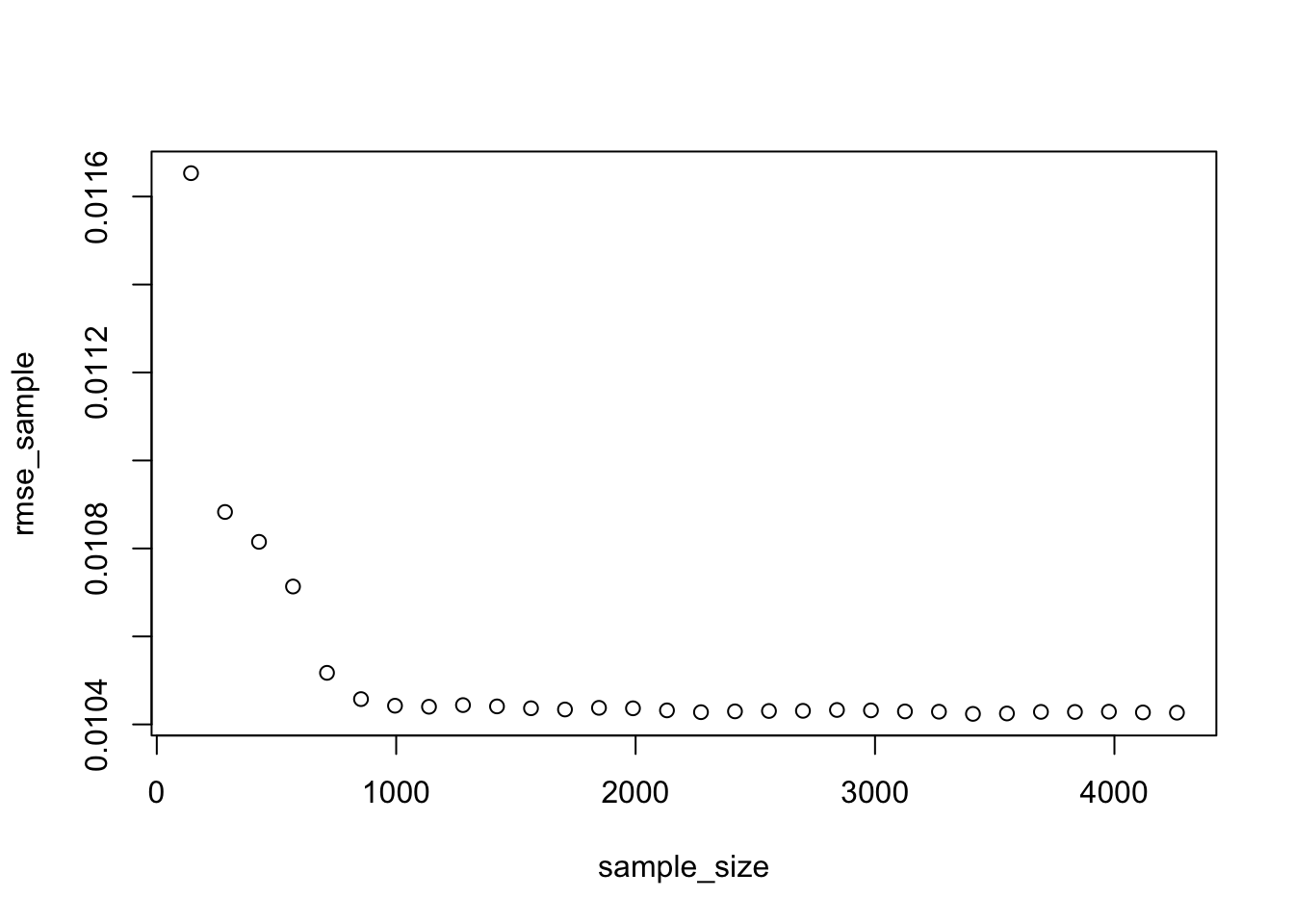
plot(sample_size,Rsq_sample)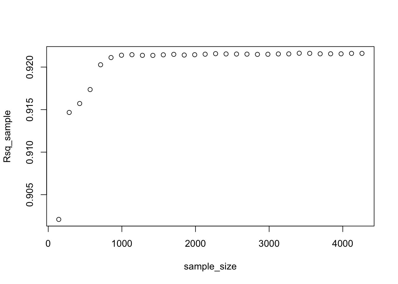
set.seed(124455454)
train_test_split <- initial_split(lc_clean, prop = 0.75)
remaining <- training(train_test_split)
testing <- testing(train_test_split)
#We are now going to run 30 models starting from a tiny training set drawn from the training data and progressively increasing its size. The testing set remains the same in all iterations.
#initiating the model by setting some parameters to zero
rmse_sample <- 0
sample_size<-0
Rsq_sample<-0
for(i in 1:30) {
#from the remaining dataset select a smaller subset to training the data
set.seed(100)
sample
learning_split <- initial_split(remaining, prop = i/200)
training <- training(learning_split)
sample_size[i]=nrow(training)
#traing the model on the small dataset
model3<-lm(int_rate ~ loan_amnt + term+ dti + annual_inc + grade + grade:loan_amnt, training)
#test the performance of the model on the large testing dataset. This stays fixed for all iterations.
pred<-predict(model3,testing)
rmse_sample[i]<-RMSE(pred,testing$int_rate)
Rsq_sample[i]<-R2(pred,testing$int_rate)
}## Warning in predict.lm(model3, testing): prediction from a rank-deficient fit may
## be misleading
## Warning in predict.lm(model3, testing): prediction from a rank-deficient fit may
## be misleading
## Warning in predict.lm(model3, testing): prediction from a rank-deficient fit may
## be misleadingplot(sample_size,rmse_sample)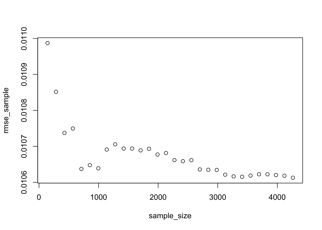
plot(sample_size,Rsq_sample)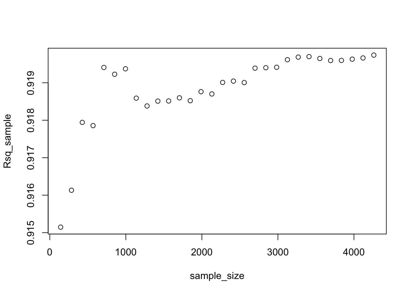
Q6. Question on learning curves
Using the learning curves above, approximately how large of a sample size would we need to estimate model 3 reliably? Once we reach this sample size, if we want to reduce the prediction error further what options do we have?
As n increases the model estimation will become more reliable and we expect the root mean square error (RMSE) of out of sample predictions to decrease and the out of sample R-squared to increase. For some n large enough, there will be little further gains from increasing n. In other words, to continue improving the performance of the model collecting more rows of the same features will not help. In the first example (set.seed(12)) we find this threshold to be approx. 1000, indicating a sample size of 1000 would be enough to estimate model 3 reliably. However, this is subject to the set seed as we see that setting the seed at 124455454 significantly changes the picture and the resulting threshold. Here, the learning curve indicates that we would need a sample size of around 3400 or perhaps >4000 to estimate model 3 reliably with smallest possible RMSE and highest possible R-squared. Taking these differences into account, we would recommend a sample size of at least 3000, potentially even around 4200 to estimate model 3 reliably.
Once we would reach this sample size, instead of increasing the sample size and reducing prediction error we will need more features/more variables or would have to try transformations of the independent and/or dependent variables in order to further improve the model’s accuracy. Another option to enhance the model’s prediction accuracy is to use a regularization method such as LASSO.
Regularization using LASSO regression
If we are in the region of the learning curve where we do not have enough data, one option is to use a regularization method such as LASSO.
We try to estimate large and complicated model (many interactions and polynomials) on a small training dataset using OLS regression and hold-out validation method.
#split the data in testing and training. The training test is really small.
set.seed(1234)
train_test_split <- initial_split(lc_clean, prop = 0.01)
training <- training(train_test_split)
testing <- testing(train_test_split)

model_lm<-lm(int_rate ~ poly(loan_amnt,3) + term+ dti + annual_inc + grade +grade:poly(loan_amnt,3):term +poly(loan_amnt,3):term +grade:term, training)
predictions <- predict(model_lm,testing)
## Warning in predict.lm(model_lm, testing): prediction from a rank-deficient fit
## may be misleading# Model prediction performance
data.frame(
RMSE = RMSE(predictions, testing$int_rate),
Rsquare = R2(predictions, testing$int_rate)
)| RMSE | Rsquare |
|---|---|
| 0.0446 | 0.352 |
Not surprisingly this model does not perform well – as we knew form the learning curves we constructed for a simpler model we need a lot more data to estimate this model reliably. Try running it again with different seeds. The model’s performance tends to be sensitive to the choice of the training set.
LASSO regression offers one solution – it extends the OLS regression by penalizing the model for setting any coefficient to a value that is different from zero. The penalty is proportional to a parameter $$ (pronounced lambda). This parameter cannot be estimated directly (and for this reason sometimes it is referred to as hyperparameter) and will be selected through k-fold cross validation in order to provide the best out-of-sample performance. As result of the LASSO procedure, only those features that are more strongly associated with the outcome will have non-zero coefficients and the estimated model will be less sensitive to the training set. Sometimes LASSO regression is referred to as regularization.
# set a seed to establish consistent results
set.seed(9999)
#we will look for the optimal lambda in this sequence (we will try 1000 different lambdas)
lambda_seq <- seq(0, 0.01, length = 1000)
#lasso regression using k-fold cross validation to select the best lambda
lasso <- train(
int_rate ~ poly(loan_amnt,3) + term+ dti + annual_inc + grade +grade:poly(loan_amnt,3):term +poly(loan_amnt,3):term +grade:term,
data = training,
method = "glmnet",
preProc = c("center", "scale"), #This option standardizes the data before running the LASSO regression
trControl = control,
tuneGrid = expand.grid(alpha = 1, lambda = lambda_seq) #alpha=1 specifies to run a LASSO regression. If alpha=0 the model would run ridge regression.
)## + Fold01: alpha=1, lambda=0.01
## - Fold01: alpha=1, lambda=0.01
## + Fold02: alpha=1, lambda=0.01
## - Fold02: alpha=1, lambda=0.01
## + Fold03: alpha=1, lambda=0.01
## - Fold03: alpha=1, lambda=0.01
## + Fold04: alpha=1, lambda=0.01
## - Fold04: alpha=1, lambda=0.01
## + Fold05: alpha=1, lambda=0.01
## - Fold05: alpha=1, lambda=0.01
## + Fold06: alpha=1, lambda=0.01
## - Fold06: alpha=1, lambda=0.01
## + Fold07: alpha=1, lambda=0.01
## - Fold07: alpha=1, lambda=0.01
## + Fold08: alpha=1, lambda=0.01
## - Fold08: alpha=1, lambda=0.01
## + Fold09: alpha=1, lambda=0.01
## - Fold09: alpha=1, lambda=0.01
## + Fold10: alpha=1, lambda=0.01
## - Fold10: alpha=1, lambda=0.01
## Aggregating results
## Selecting tuning parameters
## Fitting alpha = 1, lambda = 0.000501 on full training set# Model coefficients
coef(lasso$finalModel, lasso$bestTune$lambda)## 58 x 1 sparse Matrix of class "dgCMatrix"
## 1
## (Intercept) 1.185298e-01
## poly(loan_amnt, 3)1 .
## poly(loan_amnt, 3)2 .
## poly(loan_amnt, 3)3 .
## term60 6.322288e-04
## dti 8.026590e-07
## annual_inc .
## gradeB 1.447430e-02
## gradeC 2.309660e-02
## gradeD 2.452260e-02
## gradeE 2.285761e-02
## gradeF 1.704509e-02
## gradeG 7.944121e-03
## poly(loan_amnt, 3)1:term60 1.801161e-03
## poly(loan_amnt, 3)2:term60 .
## poly(loan_amnt, 3)3:term60 .
## term60:gradeB .
## term60:gradeC .
## term60:gradeD 2.055987e-04
## term60:gradeE 3.585581e-03
## term60:gradeF 2.199648e-04
## term60:gradeG 3.787368e-04
## poly(loan_amnt, 3)1:term36:gradeB .
## poly(loan_amnt, 3)2:term36:gradeB .
## poly(loan_amnt, 3)3:term36:gradeB .
## poly(loan_amnt, 3)1:term60:gradeB 2.624966e-05
## poly(loan_amnt, 3)2:term60:gradeB .
## poly(loan_amnt, 3)3:term60:gradeB -7.846279e-06
## poly(loan_amnt, 3)1:term36:gradeC -1.502526e-04
## poly(loan_amnt, 3)2:term36:gradeC .
## poly(loan_amnt, 3)3:term36:gradeC .
## poly(loan_amnt, 3)1:term60:gradeC -3.997393e-04
## poly(loan_amnt, 3)2:term60:gradeC .
## poly(loan_amnt, 3)3:term60:gradeC .
## poly(loan_amnt, 3)1:term36:gradeD -2.698632e-04
## poly(loan_amnt, 3)2:term36:gradeD .
## poly(loan_amnt, 3)3:term36:gradeD 4.498381e-05
## poly(loan_amnt, 3)1:term60:gradeD .
## poly(loan_amnt, 3)2:term60:gradeD .
## poly(loan_amnt, 3)3:term60:gradeD .
## poly(loan_amnt, 3)1:term36:gradeE .
## poly(loan_amnt, 3)2:term36:gradeE 2.136666e-04
## poly(loan_amnt, 3)3:term36:gradeE -3.527167e-04
## poly(loan_amnt, 3)1:term60:gradeE 2.561225e-04
## poly(loan_amnt, 3)2:term60:gradeE .
## poly(loan_amnt, 3)3:term60:gradeE 2.783084e-04
## poly(loan_amnt, 3)1:term36:gradeF .
## poly(loan_amnt, 3)2:term36:gradeF .
## poly(loan_amnt, 3)3:term36:gradeF .
## poly(loan_amnt, 3)1:term60:gradeF 1.217314e-04
## poly(loan_amnt, 3)2:term60:gradeF .
## poly(loan_amnt, 3)3:term60:gradeF .
## poly(loan_amnt, 3)1:term36:gradeG .
## poly(loan_amnt, 3)2:term36:gradeG .
## poly(loan_amnt, 3)3:term36:gradeG .
## poly(loan_amnt, 3)1:term60:gradeG 4.895644e-06
## poly(loan_amnt, 3)2:term60:gradeG 7.613254e-08
## poly(loan_amnt, 3)3:term60:gradeG .#Best lambda
lasso$bestTune$lambda## [1] 0.0005005005# Count of how many coefficients are greater than zero and how many are equal to zero
sum(coef(lasso$finalModel, lasso$bestTune$lambda)!=0)## [1] 27#sum(coef(lasso$finalModel, lasso$bestTune$lambda)>0) =22 checks strictly greater than
#sum(coef(lasso$finalModel, lasso$bestTune$lambda)<0)= 5 checks strictly less than
sum(coef(lasso$finalModel, lasso$bestTune$lambda)==0)## [1] 31# Make predictions
predictions <- predict(lasso,testing)
# Model prediction performance
data.frame(
  RMSE = RMSE(predictions, testing$int_rate),
  Rsquare = R2(predictions, testing$int_rate)
)| RMSE | Rsquare |
|---|---|
| 0.0109 | 0.918 |
Q7. Questions on LASSO regression
- Which model performs best out of sample, OLS regression or LASSO?
- What value of lambda offers best performance? Is this sensitive to the random seed?
- How many coefficients are zero and how many are non-zero in the LASSO model of best fit?
- Why is it important to standardize continuous variables before running LASSO?
These results are subject to the seed that we set in the beginning of the LASSO regression.
- The OLS yields an out of sample RMSE of 0.0445857 and an R-squared of 0.3516455 while the LASSO method yields an RMSE of 0.01086846 and R-squared of 0.9176526. Comparing those, the OLS RMSE is much larger than that of the LASSO model, while, consequently, the R-squared of the LASSO model is significantly larger than the OLS R-squared. This implies that the LASSO regression explains significantly more variance and decreases the prediction error further, meaning that the LASSO method performs better than the OLS method due to a smaller RMSE and higher R-squared.
- The best lamda is 0.0005005005, re-running the chunk without a seed or with a different seed will yield a different result, so this value is sensitive to the random seed.
- The number of coefficients that are not equal to zero is 27 (22 greater than zero and 5 less than zero), while the total number of coeffiecients equal to zero is 31.
- Coefficients of different variables are expressed and measured in different units/at different scales and therefore, we need to standardize the continous, independent variables by subtracting the mean and dividing by the standard deviation. LASSO puts constraints on the coefficient’s size so that the results depend on the magnitude of each variable. The goal is to rescale an original variable so that we can work with an equal variances/ranges across variables. Otherwise results could be misleading.
Using Time Information
Let’s try to further improve the model’s predictive performance. So far we have not used any time series information. Effectively, all things being equal, our prediction for the interest rate of a loan given in 2009 would be the same as that of a loan given in 2011. Is this a good assumption?
First, we investigate graphically whether there are any time trends in the interest rates. (Note that the variable “issue_d” only has information on the month the loan was awarded but not the exact date.) Can we use this information to further improve the forecasting accuracy of our model? Try controlling for time in a linear fashion (i.e., a linear time trend) and controlling for time as quarter dummies (this is a method to capture non-linear effects of time – we assume that the impact of time doesn’t change within a quarter but it can chance from quarter to quarter). Finally, check if time affect loans of different grades differently.
#linear time trend (add code below)
ggplot(lc_clean, aes(x=issue_d,y=int_rate))+
  geom_point(size = 0.1, alpha = 0.5)+
  geom_smooth(method = "lm", se = 0)+
  theme_bw()+
  scale_y_continuous(labels=scales::percent)+
   labs(
    title = "Higher interest rates over time (?)",
    x= "Loan issuance month",
    y="Interest rate"
  )+
  NULL
## `geom_smooth()` using formula 'y ~ x'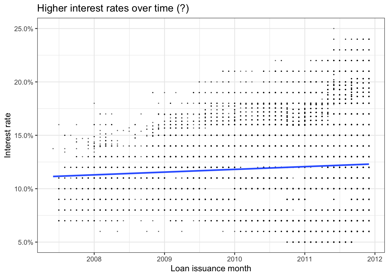
#linear time trend by grade (add code below)
ggplot(lc_clean, aes(x=issue_d,y=int_rate, color=grade))+
    geom_point(size = 0.1, alpha = 0.5)+
  geom_smooth(method = "lm", se = 0)+
  theme_bw()+
  scale_y_continuous(labels=scales::percent)+
   labs(
    title = "Higher interest rates over time? - Not for grade A",
    x= "Loan issuance month",
    y="Interest rate",
    color = "Grade"
  )+
  NULL
## `geom_smooth()` using formula 'y ~ x'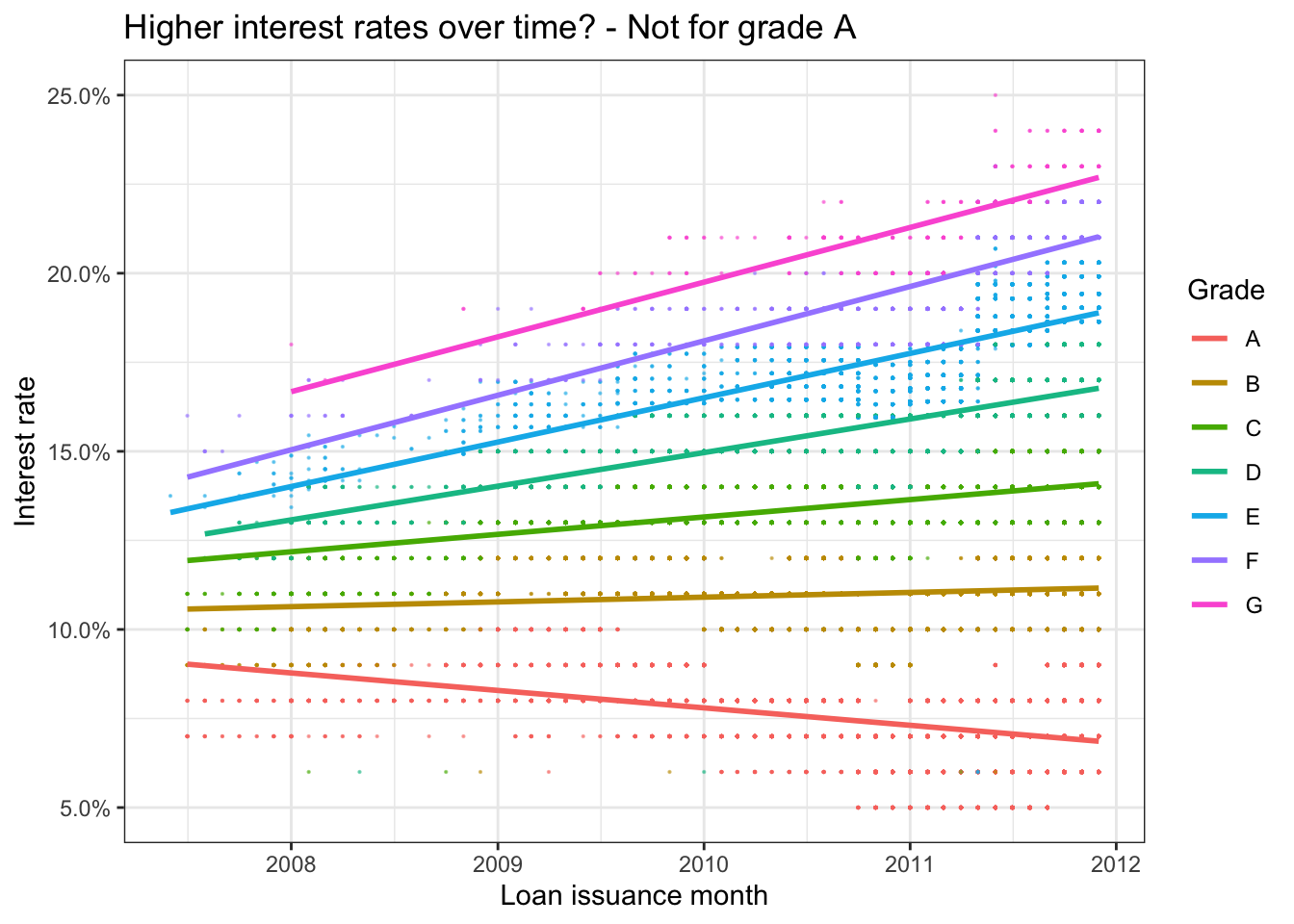
#Train models using OLS regression and k-fold cross-validation
#The first model has some explanatory variables and a linear time trend

time1<-train(
  int_rate ~ loan_amnt + term + dti + annual_inc + grade + issue_d,# using model 1 + issue_d
  lc_clean,
  method = "lm",
  trControl = control)
## + Fold01: intercept=TRUE
## - Fold01: intercept=TRUE
## + Fold02: intercept=TRUE
## - Fold02: intercept=TRUE
## + Fold03: intercept=TRUE
## - Fold03: intercept=TRUE
## + Fold04: intercept=TRUE
## - Fold04: intercept=TRUE
## + Fold05: intercept=TRUE
## - Fold05: intercept=TRUE
## + Fold06: intercept=TRUE
## - Fold06: intercept=TRUE
## + Fold07: intercept=TRUE
## - Fold07: intercept=TRUE
## + Fold08: intercept=TRUE
## - Fold08: intercept=TRUE
## + Fold09: intercept=TRUE
## - Fold09: intercept=TRUE
## + Fold10: intercept=TRUE
## - Fold10: intercept=TRUE
## Aggregating results
## Fitting final model on full training setsummary(time1)##
## Call:
## lm(formula = .outcome ~ ., data = dat)
##
## Residuals:
## Min 1Q Median 3Q Max
## -0.118129 -0.006682 -0.000625 0.007012 0.034592
##
## Coefficients:
## Estimate Std. Error t value Pr(>|t|)
## (Intercept) -2.643e-02 2.518e-03 -10.496 <2e-16 ***
## loan_amnt 1.283e-07 8.137e-09 15.772 <2e-16 ***
## term60 2.094e-03 1.444e-04 14.502 <2e-16 ***
## dti 1.485e-05 8.140e-06 1.824 0.0681 .
## annual_inc -9.230e-10 9.101e-10 -1.014 0.3105
## gradeB 3.602e-02 1.468e-04 245.430 <2e-16 ***
## gradeC 6.108e-02 1.643e-04 371.772 <2e-16 ***
## gradeD 8.263e-02 1.883e-04 438.768 <2e-16 ***
## gradeE 1.010e-01 2.449e-04 412.500 <2e-16 ***
## gradeF 1.205e-01 3.611e-04 333.813 <2e-16 ***
## gradeG 1.366e-01 6.093e-04 224.157 <2e-16 ***
## issue_d 6.606e-06 1.692e-07 39.051 <2e-16 ***
## ---
## Signif. codes: 0 '***' 0.001 '**' 0.01 '*' 0.05 '.' 0.1 ' ' 1
##
## Residual standard error: 0.01035 on 37857 degrees of freedom
## Multiple R-squared: 0.9229, Adjusted R-squared: 0.9228
## F-statistic: 4.118e+04 on 11 and 37857 DF, p-value: < 2.2e-16#The second model has a different linear time trend for each grade class
time2<-train(
int_rate ~ loan_amnt + term + dti + annual_inc + grade + issue_d + grade*issue_d, # adding interaction term between issue date and grade
lc_clean,
method = "lm",
trControl = control
)## + Fold01: intercept=TRUE
## - Fold01: intercept=TRUE
## + Fold02: intercept=TRUE
## - Fold02: intercept=TRUE
## + Fold03: intercept=TRUE
## - Fold03: intercept=TRUE
## + Fold04: intercept=TRUE
## - Fold04: intercept=TRUE
## + Fold05: intercept=TRUE
## - Fold05: intercept=TRUE
## + Fold06: intercept=TRUE
## - Fold06: intercept=TRUE
## + Fold07: intercept=TRUE
## - Fold07: intercept=TRUE
## + Fold08: intercept=TRUE
## - Fold08: intercept=TRUE
## + Fold09: intercept=TRUE
## - Fold09: intercept=TRUE
## + Fold10: intercept=TRUE
## - Fold10: intercept=TRUE
## Aggregating results
## Fitting final model on full training setsummary(time2)##
## Call:
## lm(formula = .outcome ~ ., data = dat)
##
## Residuals:
## Min 1Q Median 3Q Max
## -0.120472 -0.006447 -0.000253 0.006958 0.030466
##
## Coefficients:
## Estimate Std. Error t value Pr(>|t|)
## (Intercept) 2.802e-01 4.336e-03 64.620 < 2e-16 ***
## loan_amnt 1.312e-07 7.145e-09 18.358 < 2e-16 ***
## term60 -7.969e-04 1.295e-04 -6.155 7.60e-10 ***
## dti 5.279e-05 7.145e-06 7.388 1.52e-13 ***
## annual_inc -1.374e-09 7.979e-10 -1.722 0.0851 .
## gradeB -2.249e-01 5.799e-03 -38.791 < 2e-16 ***
## gradeC -3.440e-01 6.157e-03 -55.880 < 2e-16 ***
## gradeD -5.101e-01 7.176e-03 -71.090 < 2e-16 ***
## gradeE -6.100e-01 9.721e-03 -62.754 < 2e-16 ***
## gradeF -7.055e-01 1.572e-02 -44.872 < 2e-16 ***
## gradeG -6.942e-01 3.248e-02 -21.370 < 2e-16 ***
## issue_d -1.394e-05 2.908e-07 -47.940 < 2e-16 ***
## `gradeB:issue_d` 1.750e-05 3.884e-07 45.050 < 2e-16 ***
## `gradeC:issue_d` 2.719e-05 4.132e-07 65.807 < 2e-16 ***
## `gradeD:issue_d` 3.979e-05 4.813e-07 82.660 < 2e-16 ***
## `gradeE:issue_d` 4.768e-05 6.506e-07 73.276 < 2e-16 ***
## `gradeF:issue_d` 5.529e-05 1.049e-06 52.709 < 2e-16 ***
## `gradeG:issue_d` 5.562e-05 2.167e-06 25.672 < 2e-16 ***
## ---
## Signif. codes: 0 '***' 0.001 '**' 0.01 '*' 0.05 '.' 0.1 ' ' 1
##
## Residual standard error: 0.009073 on 37851 degrees of freedom
## Multiple R-squared: 0.9407, Adjusted R-squared: 0.9407
## F-statistic: 3.535e+04 on 17 and 37851 DF, p-value: < 2.2e-16#Change the time trend to a quarter dummy variables.
#zoo::as.yearqrt() creates quarter dummies
lc_clean_quarter<-lc_clean %>%
mutate(yq = as.factor(as.yearqtr(lc_clean$issue_d, format = "%Y-%m-%d")))
time3<-train(
int_rate ~ loan_amnt + term + dti + annual_inc + grade + yq, #using model 1 + quarter dummy variable
lc_clean_quarter,
method = "lm",
trControl = control
)## + Fold01: intercept=TRUE
## - Fold01: intercept=TRUE
## + Fold02: intercept=TRUE
## - Fold02: intercept=TRUE
## + Fold03: intercept=TRUE
## - Fold03: intercept=TRUE
## + Fold04: intercept=TRUE
## - Fold04: intercept=TRUE
## + Fold05: intercept=TRUE
## - Fold05: intercept=TRUE
## + Fold06: intercept=TRUE
## - Fold06: intercept=TRUE
## + Fold07: intercept=TRUE
## - Fold07: intercept=TRUE
## + Fold08: intercept=TRUE## Warning in predict.lm(modelFit, newdata): prediction from a rank-deficient fit
## may be misleading## - Fold08: intercept=TRUE
## + Fold09: intercept=TRUE
## - Fold09: intercept=TRUE
## + Fold10: intercept=TRUE
## - Fold10: intercept=TRUE
## Aggregating results
## Fitting final model on full training setsummary(time3)##
## Call:
## lm(formula = .outcome ~ ., data = dat)
##
## Residuals:
## Min 1Q Median 3Q Max
## -0.117045 -0.005529 -0.000010 0.005971 0.035453
##
## Coefficients:
## Estimate Std. Error t value Pr(>|t|)
## (Intercept) 3.654e-02 9.124e-03 4.005 6.22e-05 ***
## loan_amnt 6.788e-08 7.233e-09 9.385 < 2e-16 ***
## term60 4.334e-03 1.304e-04 33.244 < 2e-16 ***
## dti 1.046e-05 7.177e-06 1.458 0.144831
## annual_inc 3.866e-10 8.025e-10 0.482 0.629984
## gradeB 3.552e-02 1.296e-04 274.046 < 2e-16 ***
## gradeC 6.028e-02 1.451e-04 415.442 < 2e-16 ***
## gradeD 8.192e-02 1.663e-04 492.613 < 2e-16 ***
## gradeE 1.003e-01 2.161e-04 464.152 < 2e-16 ***
## gradeF 1.200e-01 3.185e-04 376.925 < 2e-16 ***
## gradeG 1.367e-01 5.371e-04 254.495 < 2e-16 ***
## `yq2007 Q3` 2.099e-02 9.185e-03 2.285 0.022311 *
## `yq2007 Q4` 1.667e-02 9.153e-03 1.821 0.068608 .
## `yq2008 Q1` 2.310e-02 9.131e-03 2.529 0.011432 *
## `yq2008 Q2` 2.483e-02 9.140e-03 2.717 0.006598 **
## `yq2008 Q3` 2.596e-02 9.150e-03 2.837 0.004558 **
## `yq2008 Q4` 3.374e-02 9.132e-03 3.695 0.000221 ***
## `yq2009 Q1` 3.787e-02 9.129e-03 4.148 3.36e-05 ***
## `yq2009 Q2` 3.977e-02 9.128e-03 4.356 1.33e-05 ***
## `yq2009 Q3` 4.126e-02 9.127e-03 4.521 6.17e-06 ***
## `yq2009 Q4` 4.155e-02 9.126e-03 4.553 5.30e-06 ***
## `yq2010 Q1` 3.651e-02 9.125e-03 4.001 6.32e-05 ***
## `yq2010 Q2` 3.528e-02 9.125e-03 3.866 0.000111 ***
## `yq2010 Q3` 3.638e-02 9.125e-03 3.987 6.70e-05 ***
## `yq2010 Q4` 2.775e-02 9.125e-03 3.041 0.002362 **
## `yq2011 Q1` 2.992e-02 9.124e-03 3.279 0.001042 **
## `yq2011 Q2` 3.505e-02 9.124e-03 3.841 0.000123 ***
## `yq2011 Q3` 3.744e-02 9.124e-03 4.104 4.08e-05 ***
## `yq2011 Q4` 4.370e-02 9.124e-03 4.790 1.67e-06 ***
## ---
## Signif. codes: 0 '***' 0.001 '**' 0.01 '*' 0.05 '.' 0.1 ' ' 1
##
## Residual standard error: 0.009121 on 37840 degrees of freedom
## Multiple R-squared: 0.9401, Adjusted R-squared: 0.9401
## F-statistic: 2.122e+04 on 28 and 37840 DF, p-value: < 2.2e-16#We specify one quarter dummy variable for each grade. This is going to be a large model as there are 19 quarters x 7 grades = 133 quarter-grade dummies.
time4<-train(
int_rate ~ loan_amnt + term + dti + annual_inc + grade + yq + grade*yq,
lc_clean_quarter,
method = "lm",
trControl = control
)## + Fold01: intercept=TRUE## Warning in predict.lm(modelFit, newdata): prediction from a rank-deficient fit
## may be misleading## - Fold01: intercept=TRUE
## + Fold02: intercept=TRUE## Warning in predict.lm(modelFit, newdata): prediction from a rank-deficient fit
## may be misleading## - Fold02: intercept=TRUE
## + Fold03: intercept=TRUE## Warning in predict.lm(modelFit, newdata): prediction from a rank-deficient fit
## may be misleading## - Fold03: intercept=TRUE
## + Fold04: intercept=TRUE## Warning in predict.lm(modelFit, newdata): prediction from a rank-deficient fit
## may be misleading## - Fold04: intercept=TRUE
## + Fold05: intercept=TRUE## Warning in predict.lm(modelFit, newdata): prediction from a rank-deficient fit
## may be misleading## - Fold05: intercept=TRUE
## + Fold06: intercept=TRUE## Warning in predict.lm(modelFit, newdata): prediction from a rank-deficient fit
## may be misleading## - Fold06: intercept=TRUE
## + Fold07: intercept=TRUE## Warning in predict.lm(modelFit, newdata): prediction from a rank-deficient fit
## may be misleading## - Fold07: intercept=TRUE
## + Fold08: intercept=TRUE## Warning in predict.lm(modelFit, newdata): prediction from a rank-deficient fit
## may be misleading## - Fold08: intercept=TRUE
## + Fold09: intercept=TRUE## Warning in predict.lm(modelFit, newdata): prediction from a rank-deficient fit
## may be misleading## - Fold09: intercept=TRUE
## + Fold10: intercept=TRUE## Warning in predict.lm(modelFit, newdata): prediction from a rank-deficient fit
## may be misleading## - Fold10: intercept=TRUE
## Aggregating results
## Fitting final model on full training setsummary(time4)##
## Call:
## lm(formula = .outcome ~ ., data = dat)
##
## Residuals:
## Min 1Q Median 3Q Max
## -0.120415 -0.005085 0.000519 0.004397 0.033905
##
## Coefficients: (11 not defined because of singularities)
## Estimate Std. Error t value Pr(>|t|)
## (Intercept) 2.071e-02 7.612e-03 2.720 0.006528 **
## loan_amnt 6.947e-08 6.076e-09 11.434 < 2e-16 ***
## term60 1.477e-03 1.124e-04 13.139 < 2e-16 ***
## dti 4.549e-05 6.003e-06 7.578 3.58e-14 ***
## annual_inc -1.050e-10 6.698e-10 -0.157 0.875379
## gradeB 4.059e-02 2.547e-04 159.408 < 2e-16 ***
## gradeC 6.566e-02 2.930e-04 224.089 < 2e-16 ***
## gradeD 9.508e-02 3.375e-04 281.716 < 2e-16 ***
## gradeE 1.156e-01 4.009e-04 288.419 < 2e-16 ***
## gradeF 1.364e-01 5.809e-04 234.864 < 2e-16 ***
## gradeG 1.553e-01 1.143e-03 135.892 < 2e-16 ***
## `yq2007 Q3` 5.381e-02 7.757e-03 6.938 4.05e-12 ***
## `yq2007 Q4` 5.506e-02 7.746e-03 7.108 1.20e-12 ***
## `yq2008 Q1` 5.885e-02 7.651e-03 7.691 1.49e-14 ***
## `yq2008 Q2` 6.011e-02 7.686e-03 7.821 5.37e-15 ***
## `yq2008 Q3` 5.946e-02 7.723e-03 7.700 1.39e-14 ***
## `yq2008 Q4` 6.610e-02 7.651e-03 8.640 < 2e-16 ***
## `yq2009 Q1` 6.789e-02 7.633e-03 8.894 < 2e-16 ***
## `yq2009 Q2` 6.736e-02 7.627e-03 8.831 < 2e-16 ***
## `yq2009 Q3` 6.558e-02 7.624e-03 8.601 < 2e-16 ***
## `yq2009 Q4` 6.355e-02 7.622e-03 8.339 < 2e-16 ***
## `yq2010 Q1` 5.666e-02 7.621e-03 7.434 1.07e-13 ***
## `yq2010 Q2` 5.469e-02 7.618e-03 7.179 7.17e-13 ***
## `yq2010 Q3` 5.459e-02 7.617e-03 7.167 7.82e-13 ***
## `yq2010 Q4` 4.410e-02 7.616e-03 5.791 7.05e-09 ***
## `yq2011 Q1` 4.550e-02 7.615e-03 5.974 2.33e-09 ***
## `yq2011 Q2` 4.627e-02 7.615e-03 6.076 1.24e-09 ***
## `yq2011 Q3` 4.677e-02 7.614e-03 6.143 8.19e-10 ***
## `yq2011 Q4` 5.400e-02 7.610e-03 7.096 1.30e-12 ***
## `gradeB:yq2007 Q3` -2.183e-02 2.309e-03 -9.456 < 2e-16 ***
## `gradeC:yq2007 Q3` -3.373e-02 2.433e-03 -13.862 < 2e-16 ***
## `gradeD:yq2007 Q3` -5.053e-02 3.727e-03 -13.557 < 2e-16 ***
## `gradeE:yq2007 Q3` -5.590e-02 5.592e-03 -9.996 < 2e-16 ***
## `gradeF:yq2007 Q3` -6.008e-02 3.757e-03 -15.990 < 2e-16 ***
## `gradeG:yq2007 Q3` NA NA NA NA
## `gradeB:yq2007 Q4` -2.310e-02 1.957e-03 -11.804 < 2e-16 ***
## `gradeC:yq2007 Q4` -3.422e-02 1.806e-03 -18.948 < 2e-16 ***
## `gradeD:yq2007 Q4` -4.926e-02 2.078e-03 -23.702 < 2e-16 ***
## `gradeE:yq2007 Q4` -5.009e-02 2.735e-03 -18.319 < 2e-16 ***
## `gradeF:yq2007 Q4` -5.364e-02 7.757e-03 -6.915 4.75e-12 ***
## `gradeG:yq2007 Q4` NA NA NA NA
## `gradeB:yq2008 Q1` -2.211e-02 9.872e-04 -22.400 < 2e-16 ***
## `gradeC:yq2008 Q1` -3.221e-02 1.052e-03 -30.607 < 2e-16 ***
## `gradeD:yq2008 Q1` -4.485e-02 1.182e-03 -37.941 < 2e-16 ***
## `gradeE:yq2008 Q1` -5.266e-02 1.660e-03 -31.713 < 2e-16 ***
## `gradeF:yq2008 Q1` -5.571e-02 2.857e-03 -19.497 < 2e-16 ***
## `gradeG:yq2008 Q1` -6.251e-02 5.550e-03 -11.263 < 2e-16 ***
## `gradeB:yq2008 Q2` -2.172e-02 1.367e-03 -15.886 < 2e-16 ***
## `gradeC:yq2008 Q2` -3.205e-02 1.397e-03 -22.945 < 2e-16 ***
## `gradeD:yq2008 Q2` -4.649e-02 1.652e-03 -28.137 < 2e-16 ***
## `gradeE:yq2008 Q2` -5.067e-02 2.919e-03 -17.362 < 2e-16 ***
## `gradeF:yq2008 Q2` -5.745e-02 3.609e-03 -15.917 < 2e-16 ***
## `gradeG:yq2008 Q2` NA NA NA NA
## `gradeB:yq2008 Q3` -1.916e-02 1.746e-03 -10.974 < 2e-16 ***
## `gradeC:yq2008 Q3` -2.918e-02 1.673e-03 -17.436 < 2e-16 ***
## `gradeD:yq2008 Q3` -4.417e-02 2.107e-03 -20.959 < 2e-16 ***
## `gradeE:yq2008 Q3` -4.593e-02 3.014e-03 -15.239 < 2e-16 ***
## `gradeF:yq2008 Q3` -5.545e-02 4.061e-03 -13.655 < 2e-16 ***
## `gradeG:yq2008 Q3` NA NA NA NA
## `gradeB:yq2008 Q4` -1.768e-02 1.021e-03 -17.310 < 2e-16 ***
## `gradeC:yq2008 Q4` -2.938e-02 1.056e-03 -27.806 < 2e-16 ***
## `gradeD:yq2008 Q4` -4.325e-02 1.293e-03 -33.442 < 2e-16 ***
## `gradeE:yq2008 Q4` -4.857e-02 1.679e-03 -28.929 < 2e-16 ***
## `gradeF:yq2008 Q4` -5.241e-02 3.921e-03 -13.365 < 2e-16 ***
## `gradeG:yq2008 Q4` -5.394e-02 5.549e-03 -9.721 < 2e-16 ***
## `gradeB:yq2009 Q1` -1.239e-02 9.352e-04 -13.248 < 2e-16 ***
## `gradeC:yq2009 Q1` -2.368e-02 8.206e-04 -28.861 < 2e-16 ***
## `gradeD:yq2009 Q1` -3.998e-02 9.199e-04 -43.456 < 2e-16 ***
## `gradeE:yq2009 Q1` -4.371e-02 1.248e-03 -35.020 < 2e-16 ***
## `gradeF:yq2009 Q1` -4.755e-02 2.808e-03 -16.933 < 2e-16 ***
## `gradeG:yq2009 Q1` NA NA NA NA
## `gradeB:yq2009 Q2` -1.282e-02 7.264e-04 -17.656 < 2e-16 ***
## `gradeC:yq2009 Q2` -2.309e-02 7.546e-04 -30.605 < 2e-16 ***
## `gradeD:yq2009 Q2` -3.996e-02 9.271e-04 -43.107 < 2e-16 ***
## `gradeE:yq2009 Q2` -4.432e-02 1.308e-03 -33.871 < 2e-16 ***
## `gradeF:yq2009 Q2` -5.257e-02 2.414e-03 -21.779 < 2e-16 ***
## `gradeG:yq2009 Q2` -5.447e-02 3.999e-03 -13.622 < 2e-16 ***
## `gradeB:yq2009 Q3` -1.081e-02 6.353e-04 -17.008 < 2e-16 ***
## `gradeC:yq2009 Q3` -1.937e-02 6.942e-04 -27.907 < 2e-16 ***
## `gradeD:yq2009 Q3` -3.246e-02 8.763e-04 -37.043 < 2e-16 ***
## `gradeE:yq2009 Q3` -3.679e-02 1.131e-03 -32.519 < 2e-16 ***
## `gradeF:yq2009 Q3` -4.211e-02 1.847e-03 -22.795 < 2e-16 ***
## `gradeG:yq2009 Q3` -4.592e-02 3.122e-03 -14.709 < 2e-16 ***
## `gradeB:yq2009 Q4` -7.857e-03 5.673e-04 -13.848 < 2e-16 ***
## `gradeC:yq2009 Q4` -1.570e-02 6.168e-04 -25.452 < 2e-16 ***
## `gradeD:yq2009 Q4` -2.770e-02 7.071e-04 -39.175 < 2e-16 ***
## `gradeE:yq2009 Q4` -3.323e-02 1.108e-03 -30.004 < 2e-16 ***
## `gradeF:yq2009 Q4` -3.573e-02 1.701e-03 -21.010 < 2e-16 ***
## `gradeG:yq2009 Q4` -3.607e-02 2.503e-03 -14.406 < 2e-16 ***
## `gradeB:yq2010 Q1` -1.017e-02 5.418e-04 -18.775 < 2e-16 ***
## `gradeC:yq2010 Q1` -1.075e-02 6.023e-04 -17.852 < 2e-16 ***
## `gradeD:yq2010 Q1` -2.123e-02 6.862e-04 -30.937 < 2e-16 ***
## `gradeE:yq2010 Q1` -2.462e-02 1.015e-03 -24.256 < 2e-16 ***
## `gradeF:yq2010 Q1` -3.026e-02 1.796e-03 -16.844 < 2e-16 ***
## `gradeG:yq2010 Q1` -2.900e-02 3.114e-03 -9.315 < 2e-16 ***
## `gradeB:yq2010 Q2` -9.475e-03 4.815e-04 -19.678 < 2e-16 ***
## `gradeC:yq2010 Q2` -7.761e-03 5.277e-04 -14.707 < 2e-16 ***
## `gradeD:yq2010 Q2` -1.835e-02 5.943e-04 -30.873 < 2e-16 ***
## `gradeE:yq2010 Q2` -2.259e-02 7.727e-04 -29.240 < 2e-16 ***
## `gradeF:yq2010 Q2` -2.788e-02 1.307e-03 -21.327 < 2e-16 ***
## `gradeG:yq2010 Q2` -2.629e-02 2.578e-03 -10.199 < 2e-16 ***
## `gradeB:yq2010 Q3` -6.881e-03 4.615e-04 -14.910 < 2e-16 ***
## `gradeC:yq2010 Q3` -4.074e-03 5.056e-04 -8.058 8.01e-16 ***
## `gradeD:yq2010 Q3` -1.661e-02 5.665e-04 -29.319 < 2e-16 ***
## `gradeE:yq2010 Q3` -2.326e-02 6.711e-04 -34.663 < 2e-16 ***
## `gradeF:yq2010 Q3` -2.671e-02 1.070e-03 -24.967 < 2e-16 ***
## `gradeG:yq2010 Q3` -2.441e-02 1.875e-03 -13.016 < 2e-16 ***
## `gradeB:yq2010 Q4` -7.631e-03 4.287e-04 -17.801 < 2e-16 ***
## `gradeC:yq2010 Q4` -5.675e-04 4.823e-04 -1.177 0.239305
## `gradeD:yq2010 Q4` -1.276e-02 5.571e-04 -22.910 < 2e-16 ***
## `gradeE:yq2010 Q4` -1.664e-02 6.685e-04 -24.885 < 2e-16 ***
## `gradeF:yq2010 Q4` -1.935e-02 1.040e-03 -18.603 < 2e-16 ***
## `gradeG:yq2010 Q4` -1.879e-02 1.672e-03 -11.239 < 2e-16 ***
## `gradeB:yq2011 Q1` -5.344e-03 4.114e-04 -12.990 < 2e-16 ***
## `gradeC:yq2011 Q1` -1.646e-03 4.738e-04 -3.474 0.000514 ***
## `gradeD:yq2011 Q1` -1.028e-02 5.287e-04 -19.453 < 2e-16 ***
## `gradeE:yq2011 Q1` -1.534e-02 6.065e-04 -25.292 < 2e-16 ***
## `gradeF:yq2011 Q1` -1.767e-02 8.504e-04 -20.783 < 2e-16 ***
## `gradeG:yq2011 Q1` -2.010e-02 1.525e-03 -13.184 < 2e-16 ***
## `gradeB:yq2011 Q2` -7.395e-04 3.912e-04 -1.891 0.058684 .
## `gradeC:yq2011 Q2` 1.166e-03 4.423e-04 2.636 0.008399 **
## `gradeD:yq2011 Q2` -3.678e-03 4.950e-04 -7.431 1.10e-13 ***
## `gradeE:yq2011 Q2` -5.008e-03 5.847e-04 -8.565 < 2e-16 ***
## `gradeF:yq2011 Q2` -4.529e-03 8.391e-04 -5.398 6.79e-08 ***
## `gradeG:yq2011 Q2` -1.004e-02 1.587e-03 -6.326 2.55e-10 ***
## `gradeB:yq2011 Q3` 1.563e-03 3.666e-04 4.262 2.03e-05 ***
## `gradeC:yq2011 Q3` 2.724e-03 4.239e-04 6.427 1.32e-10 ***
## `gradeD:yq2011 Q3` -1.597e-04 4.765e-04 -0.335 0.737471
## `gradeE:yq2011 Q3` 1.813e-03 5.786e-04 3.133 0.001729 **
## `gradeF:yq2011 Q3` 1.180e-03 8.613e-04 1.370 0.170744
## `gradeG:yq2011 Q3` -7.748e-04 1.616e-03 -0.479 0.631681
## `gradeB:yq2011 Q4` NA NA NA NA
## `gradeC:yq2011 Q4` NA NA NA NA
## `gradeD:yq2011 Q4` NA NA NA NA
## `gradeE:yq2011 Q4` NA NA NA NA
## `gradeF:yq2011 Q4` NA NA NA NA
## `gradeG:yq2011 Q4` NA NA NA NA
## ---
## Signif. codes: 0 '***' 0.001 '**' 0.01 '*' 0.05 '.' 0.1 ' ' 1
##
## Residual standard error: 0.007601 on 37743 degrees of freedom
## Multiple R-squared: 0.9585, Adjusted R-squared: 0.9584
## F-statistic: 6979 on 125 and 37743 DF, p-value: < 2.2e-16data.frame(
time1$results$RMSE,
time2$results$RMSE,
time3$results$RMSE,
time4$results$RMSE)| time1.results.RMSE | time2.results.RMSE | time3.results.RMSE | time4.results.RMSE |
|---|---|---|---|
| 0.0104 | 0.00907 | 0.00913 | 0.00761 |
data.frame(
summary(time1)$adj.r.squared,
summary(time2)$adj.r.squared,
summary(time3)$adj.r.squared,
summary(time4)$adj.r.squared)| summary.time1..adj.r.squared | summary.time2..adj.r.squared | summary.time3..adj.r.squared | summary.time4..adj.r.squared |
|---|---|---|---|
| 0.923 | 0.941 | 0.94 | 0.958 |
Q8. Question on time series models
Based on our analysis above, is there any evidence to suggest that interest rates change over time? Does including time trends /quarter dummies improve predictions?
Graphically, the first graph shows a very slight increase of the interest rate over time. Differentiating interest rates by grade gives a clearer picture into the trends of interest rates over time. As we have seen before, the better the grade, the lower the interest rate overall. Additionally, we now see that the interest rates of grade A loans have actually decreased over time while the interest rates of all other loan grades have increased over time. Grade B only increases slightly, while the interest rates of lower grade loans increase more significantly, especially grades G, F and E.
Using these insights for optimizing our models, we assessed the signifiance of time (issue_d) on our previously created and preferred model (model1). In time1 we find that issue_d is statistically significant (t-value 39.051 >>|2|) this slighly improved our model’s adjusted R-squared and reduces the RMSE, improving our model overall. Including an interaction variable in time2 highlights the significance of time (issue_d) per grade as each variable is statistically significant, this again leads to an increase in explanatory power. The implementation of a dummy variable for quarters in time3 improved time1’s predictive power by an almost 2% increase. However, using the quarter dummy variable and interaction terms in time4 yields the strongest result (amongst all our models) with an RMSE of 0.007614248 and adjusted R-squared of 0.958393. Technically speaking, the time trends and even more so the quarter dummies improve our model as the RSME decreases and the adjusted R-squared increases. Considering if adding time variables to our model is sensible makes us realize that time is not a very reliable factor for prediction as it often (but most importantly not always!) correlates with eonomic conditions which can drastically change - so that real-life predictions must take into account other factors from the economic environment rather than time in order to improve those predictions. Additionally, a specific time input will not be a yield a good prediction since attempting to predict the interest rate in the future will, most probably, not depend on whether someone takes on a loan on, e.g., March 5th or Arpil 5th. While our model has improved in explaining the variance of our data, including time trends and quarter dummies is not a good way to predict future interest rates.
Using Bond Yields
One concern with using time trends for forecasting is that in order to make predictions for future loans we will need to project trends to the future. This is an extrapolation that may not be reasonable, especially if macroeconomic conditions in the future change. Furthermore, if we are using quarter dummies, it is not even possible to estimate the coefficient of these dummy variables for future quarters.
Instead, perhaps it’s better to find the reasons as to why different periods are different from one another. The csv file “MonthBondYields.csv” contains information on the yield of US Treasuries on the first day of each month.
#load the data to memory as a dataframe
bond_prices<-vroom::vroom(here::here("data", "MonthBondYields.csv"))
## New names:
## * `` -> ...7
## * `` -> ...8
## * `` -> ...9
## * `` -> ...10## Rows: 54
## Columns: 10
## Delimiter: ","
## chr [2]: Date, Change %
## dbl [4]: Price, Open, High, Low
## lgl [4]: ...7, ...8, ...9, ...10
##
## Use `spec()` to retrieve the guessed column specification
## Pass a specification to the `col_types` argument to quiet this message#make the date of the bond file comparable to the lending club dataset
#for some regional date/number (locale) settings this may not work. If it does try running the following line of code in the Console
#Sys.setlocale("LC_TIME","English")
bond_prices <- bond_prices %>%
mutate(Date2=as.Date(paste("01",Date,sep="-"),"%d-%b-%y")) %>%
select(-starts_with("X"))
#let's see what happened to bond yields over time. Lower bond yields mean the cost of borrowing has gone down.
bond_prices %>%
ggplot(aes(x=Date2, y=Price))+
geom_point(size = 0.1, alpha = 0.5)+
geom_smooth(method = "lm", se = 0)+
theme_bw()+
labs(
title = "Descreasing yields over time",
x= "Year",
y="Price"
)+
NULL## `geom_smooth()` using formula 'y ~ x'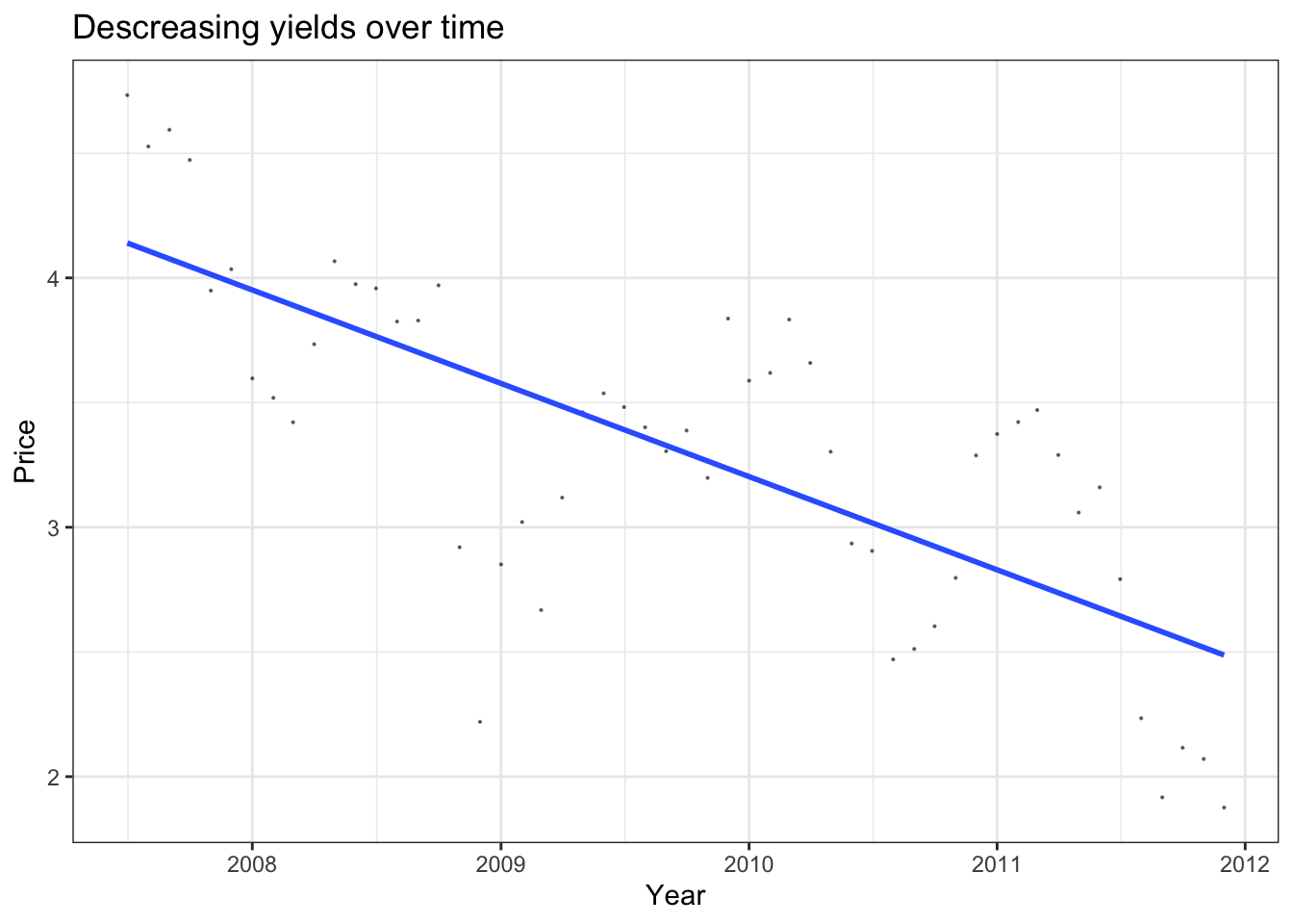
#join the data using a left join
lc_with_bonds<-lc_clean %>%
  left_join(bond_prices, by = c("issue_d" = "Date2")) %>%
  arrange(issue_d) %>%
  filter(!is.na(Price)) #drop any observations where there re no bond prices available

# investigate graphically if there is a relationship
lc_with_bonds %>%
  ggplot(aes(x=int_rate, y=Price))+
  geom_point(size = 0.1, alpha = 0.5)+
  geom_smooth(method = "lm", se = 0)+
  theme_bw()+
  scale_x_continuous(labels=scales::percent)+
   labs(
    title = "Interest rates vs. bond prices",
    x= "Interest rate",
    y="Price"
  )+
  NULL
## `geom_smooth()` using formula 'y ~ x'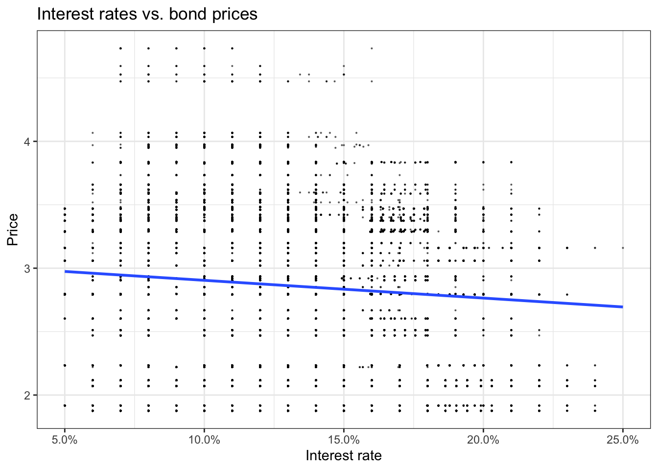
lc_with_bonds%>%
  ggplot(aes(x=int_rate, y=Price, color=grade))+
  geom_point(size=0.1, alpha=0.5)+
  geom_smooth(method="lm", se = 0) +
  theme_bw()+
  scale_x_continuous(labels=scales::percent)+
   labs(
    title = "Interest rates vs. bond prices by grade",
    x= "Interest rate",
    y="Price",
    color = "Grade"
  )+
  NULL
## `geom_smooth()` using formula 'y ~ x'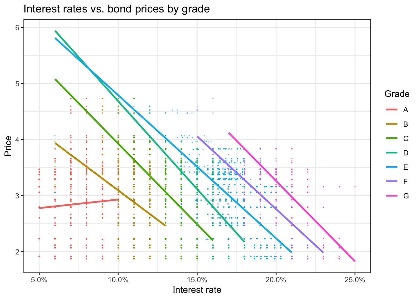
#let's train a model using the bond information


plsFit<-train(
    int_rate ~ loan_amnt+term+dti+annual_inc+grade+Price , #model 1+ price
    lc_with_bonds,
   method = "lm",
    trControl = control
   )
## + Fold01: intercept=TRUE
## - Fold01: intercept=TRUE
## + Fold02: intercept=TRUE
## - Fold02: intercept=TRUE
## + Fold03: intercept=TRUE
## - Fold03: intercept=TRUE
## + Fold04: intercept=TRUE
## - Fold04: intercept=TRUE
## + Fold05: intercept=TRUE
## - Fold05: intercept=TRUE
## + Fold06: intercept=TRUE
## - Fold06: intercept=TRUE
## + Fold07: intercept=TRUE
## - Fold07: intercept=TRUE
## + Fold08: intercept=TRUE
## - Fold08: intercept=TRUE
## + Fold09: intercept=TRUE
## - Fold09: intercept=TRUE
## + Fold10: intercept=TRUE
## - Fold10: intercept=TRUE
## Aggregating results
## Fitting final model on full training setsummary(plsFit)##
## Call:
## lm(formula = .outcome ~ ., data = dat)
##
## Residuals:
## Min 1Q Median 3Q Max
## -0.115867 -0.006443 -0.000230 0.006585 0.036982
##
## Coefficients:
## Estimate Std. Error t value Pr(>|t|)
## (Intercept) 8.734e-02 3.048e-04 286.592 <2e-16 ***
## loan_amnt 1.106e-07 7.932e-09 13.946 <2e-16 ***
## term60 2.236e-03 1.373e-04 16.283 <2e-16 ***
## dti 1.795e-05 7.906e-06 2.271 0.0232 *
## annual_inc -3.450e-10 8.863e-10 -0.389 0.6971
## gradeB 3.607e-02 1.427e-04 252.784 <2e-16 ***
## gradeC 6.100e-02 1.589e-04 383.813 <2e-16 ***
## gradeD 8.260e-02 1.826e-04 452.464 <2e-16 ***
## gradeE 1.011e-01 2.378e-04 425.059 <2e-16 ***
## gradeF 1.209e-01 3.514e-04 343.953 <2e-16 ***
## gradeG 1.371e-01 5.933e-04 231.115 <2e-16 ***
## Price -5.267e-03 8.703e-05 -60.526 <2e-16 ***
## ---
## Signif. codes: 0 '***' 0.001 '**' 0.01 '*' 0.05 '.' 0.1 ' ' 1
##
## Residual standard error: 0.01008 on 37856 degrees of freedom
## Multiple R-squared: 0.9269, Adjusted R-squared: 0.9268
## F-statistic: 4.362e+04 on 11 and 37856 DF, p-value: < 2.2e-16Q9. Question on bond yields
Do bond yields have any explanatory power?
Bond prices and yields are great indicators of the economy as a whole (in particular of inflation). Bond price and yield have an inverse relationship, meaning the higher a bond’s price, the lower its yield. By plotting
Priceand incorporating the variable into our model, we can make assumptions about the explanatory power of both bond price and yield.
By plotting bond price against time we see there is a decreasing trend of bond price over time and, after plotting Price vs. interest rate, that, thus, the cost of borrowing is actually decreasing over time, i.e we would expect lower interest rates over time. Bond prices are also a good indicator of market conditions over time and thus would incorporate information about changes over time without having to use an explicit time vector that would be very difficult to make predictions on. Exploring the relationship of Prices vs Interest rates we notice bonds have a slight inverse relationship to interest rates i.e when the cost of borrowing money rises, bond prices usually fall, and vice-versa. The first graph only demonstates that this relationship is fairly weak and might not hold over all bond types. By filtering for grade we see a much clearer invese relationship between bond price and interest rates across bond grades B-G, however we note that there is actually a positive reltionship for grade A bonds. The rational for this invese relationship is quite logical as most bonds pay a fixed interest rate that becomes more attractive if interest rates fall, driving up demand and the price of the bond. Conversely, if interest rates rise, investors will no longer prefer the lower fixed interest rate paid by a bond, resulting in a decline in its price. It is interesting to note that grade A bonds do not obey this rule and actually become more favourable with a higher interest rate, this may be due to the surety of return that grade A bonds offer.
As we can see a clear relationship exists, so we include bond prices as an explanatory variable in our model which proved to be significant (t-value = 60.526 >> |2|). This indicates that bond price and, thus, bond yields have high explanatory power for interest rates. The model also has a higher adjusted R-squared of 0.9268 and lower residual std error of 0.01008 than model1, so we can conclude that is is indeed a stronger model and reveals more meaningful results (that could be used for prediction) than the time series models (where we cannot extrapolated data into the future reliably) .
Final model
Q10. We choose a model and describe our methodology.
# final model: model1 + Price + interaction between Price and grade + eliminate annual income

finalmodel<-train(
    int_rate ~ loan_amnt+term+dti+grade+Price+ Price*grade,
    lc_with_bonds,
   method = "lm",
    trControl = control
   )
## + Fold01: intercept=TRUE
## - Fold01: intercept=TRUE
## + Fold02: intercept=TRUE
## - Fold02: intercept=TRUE
## + Fold03: intercept=TRUE
## - Fold03: intercept=TRUE
## + Fold04: intercept=TRUE
## - Fold04: intercept=TRUE
## + Fold05: intercept=TRUE
## - Fold05: intercept=TRUE
## + Fold06: intercept=TRUE
## - Fold06: intercept=TRUE
## + Fold07: intercept=TRUE
## - Fold07: intercept=TRUE
## + Fold08: intercept=TRUE
## - Fold08: intercept=TRUE
## + Fold09: intercept=TRUE
## - Fold09: intercept=TRUE
## + Fold10: intercept=TRUE
## - Fold10: intercept=TRUE
## Aggregating results
## Fitting final model on full training setsummary(finalmodel)##
## Call:
## lm(formula = .outcome ~ ., data = dat)
##
## Residuals:
## Min 1Q Median 3Q Max
## -0.119101 -0.005686 -0.000274 0.006467 0.040287
##
## Coefficients:
## Estimate Std. Error t value Pr(>|t|)
## (Intercept) 6.874e-02 4.891e-04 140.526 < 2e-16 ***
## loan_amnt 1.137e-07 7.254e-09 15.671 < 2e-16 ***
## term60 1.322e-03 1.317e-04 10.040 < 2e-16 ***
## dti 2.969e-05 7.459e-06 3.980 6.90e-05 ***
## gradeB 5.234e-02 6.362e-04 82.272 < 2e-16 ***
## gradeC 8.321e-02 7.149e-04 116.387 < 2e-16 ***
## gradeD 1.195e-01 8.226e-04 145.237 < 2e-16 ***
## gradeE 1.457e-01 1.041e-03 139.917 < 2e-16 ***
## gradeF 1.698e-01 1.534e-03 110.693 < 2e-16 ***
## gradeG 1.881e-01 2.865e-03 65.637 < 2e-16 ***
## Price 1.207e-03 1.610e-04 7.492 6.93e-14 ***
## `gradeB:Price` -5.667e-03 2.167e-04 -26.150 < 2e-16 ***
## `gradeC:Price` -7.694e-03 2.411e-04 -31.907 < 2e-16 ***
## `gradeD:Price` -1.275e-02 2.784e-04 -45.792 < 2e-16 ***
## `gradeE:Price` -1.556e-02 3.569e-04 -43.592 < 2e-16 ***
## `gradeF:Price` -1.703e-02 5.268e-04 -32.318 < 2e-16 ***
## `gradeG:Price` -1.757e-02 9.773e-04 -17.976 < 2e-16 ***
## ---
## Signif. codes: 0 '***' 0.001 '**' 0.01 '*' 0.05 '.' 0.1 ' ' 1
##
## Residual standard error: 0.009607 on 37851 degrees of freedom
## Multiple R-squared: 0.9336, Adjusted R-squared: 0.9335
## F-statistic: 3.324e+04 on 16 and 37851 DF, p-value: < 2.2e-16After investigating more models with different features using the methodologies covered so far, we present the model we believe predicts interest rates the best. We describe the chosen methodology and how good it is (including the approximate length of the 95% Confidence Interval of predictions that use this model) and what features it uses. (We do not use time trends or quarter dummies in our model as the first cannot be extrapolated into the future reliably and the second cannot be even estimated for future quarters.)
Above is the model we believe, at this point, predicts interest rates the best and most reliably as all explanatroy variables are highly significant (t-value>>|2|) and no time trends or quarter dummy variables are added.
The 95 % confidence interval for any prediction will be (+/- 2* RSE), (-0.019214, 0.019214), meaning an error width of 3.8% in interest rate estimate. This is smaller than the predicition interval in model 1. We have an adjusted R-squared of 0.9335 and residual standard error of 0.009607 which suggests very high explanatory power.
We use a 10 fold cross validation method which is not subject to random seed errors. Our model uses an interaction term between grade and bond price as we saw different relationships (question 9) between interest rates and bond price amongst different grades. We eliminated annual income as an explanatory variable as it was not statistically significant in model 1 or our final model, and we are left with a model with highly significant explanatory variables.
Q11. Exploring the effects of CPI and Inflation on the model
We use other publicly available datasets to further improve performance (e.g., quarterly data on US inflation or CPI) and explain why and check if the additional data will make a difference.
Additionaly, more data - especially more data on the economic and business environment may significantly improve our model as it provides more information that can explain more of the variance of our model.
#load data
cpi <- vroom::vroom(here::here("data", "consumerpriceindex.csv"))
## Rows: 242
## Columns: 2
## Delimiter: ","
## dbl [1]: CPALTT01USQ657N
## date [1]: DATE
##
## Use `spec()` to retrieve the guessed column specification
## Pass a specification to the `col_types` argument to quiet this messagecpi <- cpi %>%
rename(cpi = CPALTT01USQ657N)
#glimpse
glimpse(cpi)## Rows: 242
## Columns: 2
## $ DATE <date> 1960-01-01, 1960-04-01, 1960-07-01, 1960-10-01, 1961-01-01, 196…
## $ cpi <dbl> -0.1133787, 0.5675369, 0.2257336, 0.6756757, 0.0000000, 0.000000…#join the data using a left join
lc_with_bonds_cpis <- lc_with_bonds %>%
left_join(cpi, by = c("issue_d" = "DATE")) %>%
arrange(issue_d) %>%
filter(!is.na(cpi))
#add cpi as explanatory variable to our final model
finalmodel_cpi<-train(
int_rate ~ loan_amnt + term + dti + grade + Price + Price*grade + cpi, #final model with consumer price index
lc_with_bonds_cpis,
method = "lm",
trControl = control
)## + Fold01: intercept=TRUE
## - Fold01: intercept=TRUE
## + Fold02: intercept=TRUE
## - Fold02: intercept=TRUE
## + Fold03: intercept=TRUE
## - Fold03: intercept=TRUE
## + Fold04: intercept=TRUE
## - Fold04: intercept=TRUE
## + Fold05: intercept=TRUE
## - Fold05: intercept=TRUE
## + Fold06: intercept=TRUE
## - Fold06: intercept=TRUE
## + Fold07: intercept=TRUE
## - Fold07: intercept=TRUE
## + Fold08: intercept=TRUE
## - Fold08: intercept=TRUE
## + Fold09: intercept=TRUE
## - Fold09: intercept=TRUE
## + Fold10: intercept=TRUE
## - Fold10: intercept=TRUE
## Aggregating results
## Fitting final model on full training setsummary(finalmodel_cpi)##
## Call:
## lm(formula = .outcome ~ ., data = dat)
##
## Residuals:
## Min 1Q Median 3Q Max
## -0.089094 -0.005176 0.000160 0.006051 0.028324
##
## Coefficients:
## Estimate Std. Error t value Pr(>|t|)
## (Intercept) 6.251e-02 9.519e-04 65.672 < 2e-16 ***
## loan_amnt 1.294e-07 1.230e-08 10.527 < 2e-16 ***
## term60 1.069e-03 2.287e-04 4.675 2.98e-06 ***
## dti 2.436e-05 1.237e-05 1.969 0.0489 *
## gradeB 5.726e-02 1.257e-03 45.533 < 2e-16 ***
## gradeC 9.284e-02 1.419e-03 65.433 < 2e-16 ***
## gradeD 1.298e-01 1.659e-03 78.261 < 2e-16 ***
## gradeE 1.570e-01 2.110e-03 74.405 < 2e-16 ***
## gradeF 1.859e-01 3.342e-03 55.603 < 2e-16 ***
## gradeG 1.955e-01 5.955e-03 32.833 < 2e-16 ***
## Price 3.967e-03 3.145e-04 12.612 < 2e-16 ***
## cpi -3.234e-03 1.372e-04 -23.567 < 2e-16 ***
## `gradeB:Price` -7.381e-03 4.153e-04 -17.772 < 2e-16 ***
## `gradeC:Price` -1.097e-02 4.626e-04 -23.705 < 2e-16 ***
## `gradeD:Price` -1.617e-02 5.425e-04 -29.816 < 2e-16 ***
## `gradeE:Price` -1.934e-02 7.037e-04 -27.481 < 2e-16 ***
## `gradeF:Price` -2.286e-02 1.118e-03 -20.448 < 2e-16 ***
## `gradeG:Price` -2.027e-02 2.026e-03 -10.003 < 2e-16 ***
## ---
## Signif. codes: 0 '***' 0.001 '**' 0.01 '*' 0.05 '.' 0.1 ' ' 1
##
## Residual standard error: 0.009045 on 12000 degrees of freedom
## Multiple R-squared: 0.9381, Adjusted R-squared: 0.938
## F-statistic: 1.07e+04 on 17 and 12000 DF, p-value: < 2.2e-16Adding consumer price index data to our final mode, we find another model with high explanatory power with an adj R-squared of 0.938 and an residual standard error of 0.009045 - this is only marginally better than our final model and for computational purposes it may still be better to assume our previous final model as best model.
#load data
inflation <- vroom::vroom(here::here("data", "inflation.csv"))
## Rows: 60
## Columns: 2
## Delimiter: ","
## dbl [1]: FPCPITOTLZGUSA
## date [1]: DATE
##
## Use `spec()` to retrieve the guessed column specification
## Pass a specification to the `col_types` argument to quiet this messageinflation <- inflation %>%
rename(inflation = FPCPITOTLZGUSA) %>%
# create year column as inflation rates are per year
mutate(year = format(as.Date(DATE, format="%Y-%m-%d"),"%Y"))
# create year column as inflation rates are per yea
lc_with_bonds_cpis <- lc_with_bonds_cpis %>%
mutate(year = format(as.Date(issue_d, format="%Y-%m-%d"),"%Y"))
#glimpse
glimpse(inflation)## Rows: 60
## Columns: 3
## $ DATE <date> 1960-01-01, 1961-01-01, 1962-01-01, 1963-01-01, 1964-01-01…
## $ inflation <dbl> 1.457976, 1.070724, 1.198773, 1.239669, 1.278912, 1.585169,…
## $ year <chr> "1960", "1961", "1962", "1963", "1964", "1965", "1966", "19…#join the data using a left join
lc_with_bonds_cpis_inflation <- lc_with_bonds_cpis %>%
left_join(inflation, by = c("year" = "year")) %>%
arrange(issue_d) %>%
filter(!is.na(cpi))
#add inflation as explanatory variable to our final model
finalmodel_inflation <- train(
int_rate ~ loan_amnt + term + dti + grade + Price + Price*grade + inflation, #final model with inflation data
lc_with_bonds_cpis_inflation,
method = "lm",
trControl = control
)## + Fold01: intercept=TRUE
## - Fold01: intercept=TRUE
## + Fold02: intercept=TRUE
## - Fold02: intercept=TRUE
## + Fold03: intercept=TRUE
## - Fold03: intercept=TRUE
## + Fold04: intercept=TRUE
## - Fold04: intercept=TRUE
## + Fold05: intercept=TRUE
## - Fold05: intercept=TRUE
## + Fold06: intercept=TRUE
## - Fold06: intercept=TRUE
## + Fold07: intercept=TRUE
## - Fold07: intercept=TRUE
## + Fold08: intercept=TRUE
## - Fold08: intercept=TRUE
## + Fold09: intercept=TRUE
## - Fold09: intercept=TRUE
## + Fold10: intercept=TRUE
## - Fold10: intercept=TRUE
## Aggregating results
## Fitting final model on full training setsummary(finalmodel_inflation)##
## Call:
## lm(formula = .outcome ~ ., data = dat)
##
## Residuals:
## Min 1Q Median 3Q Max
## -0.089804 -0.005371 0.000307 0.005996 0.025673
##
## Coefficients:
## Estimate Std. Error t value Pr(>|t|)
## (Intercept) 7.438e-02 9.624e-04 77.282 < 2e-16 ***
## loan_amnt 1.379e-07 1.227e-08 11.242 < 2e-16 ***
## term60 1.045e-03 2.278e-04 4.585 4.59e-06 ***
## dti 2.485e-05 1.235e-05 2.013 0.0442 *
## gradeB 5.699e-02 1.255e-03 45.400 < 2e-16 ***
## gradeC 9.038e-02 1.418e-03 63.737 < 2e-16 ***
## gradeD 1.291e-01 1.657e-03 77.945 < 2e-16 ***
## gradeE 1.574e-01 2.105e-03 74.768 < 2e-16 ***
## gradeF 1.874e-01 3.334e-03 56.203 < 2e-16 ***
## gradeG 1.983e-01 5.941e-03 33.385 < 2e-16 ***
## Price 7.647e-04 3.008e-04 2.542 0.0110 *
## inflation -1.764e-03 7.193e-05 -24.526 < 2e-16 ***
## `gradeB:Price` -7.280e-03 4.146e-04 -17.558 < 2e-16 ***
## `gradeC:Price` -1.014e-02 4.619e-04 -21.963 < 2e-16 ***
## `gradeD:Price` -1.600e-02 5.417e-04 -29.545 < 2e-16 ***
## `gradeE:Price` -1.952e-02 7.021e-04 -27.798 < 2e-16 ***
## `gradeF:Price` -2.343e-02 1.115e-03 -21.020 < 2e-16 ***
## `gradeG:Price` -2.136e-02 2.021e-03 -10.568 < 2e-16 ***
## ---
## Signif. codes: 0 '***' 0.001 '**' 0.01 '*' 0.05 '.' 0.1 ' ' 1
##
## Residual standard error: 0.009028 on 12000 degrees of freedom
## Multiple R-squared: 0.9383, Adjusted R-squared: 0.9382
## F-statistic: 1.074e+04 on 17 and 12000 DF, p-value: < 2.2e-16We couldn’t significantly improve our final model by adding inflation. Adding inflation does yield a slightly lower RMSE; however, it has also made a number of other factors insignificant (factors that previously were significant). This may be due to multicolinearity or heteroskedasticity issues. The reduced RMSE does improve the predictive interval for the model however this is only marginally and for simplicity and computational sake (Occam’s Razor) We decide to not include inflation in our model.
Moving forward, we could look for further data in the economics and business environment that influences interest rates significantly to help us to further improve our model and its predictive accuracy. We could also consider a series of different transformations on the existing data we have.