Classification with Logistic Regression for the Lending Club

Introduction

Welcome to the second Lending Club data analysis. Now, we will take the perspective of an investor to the lending club. Our goal is to select a subset of the most promising loans to invest. We will do so using the method of logistic regression. Feel free to consult the R markdown file of session 4.

Load the data

First we need to start by loading the data.

lc_raw <- read_csv(here::here("data", "LendingClub Data.csv"),  skip=1) %>%  #since the first row is a title we want to skip it. 
  clean_names() # use janitor::clean_names()

ICE the data: Inspect, Clean, Explore

Any data science engagement starts with ICE. Inspecting, Clean and Explore the data.

Inspect the data

We inspect the data to understand what different variables mean.

glimpse(lc_raw)

## Rows: 42,538
## Columns: 80
## $ int_rate            <dbl> 0.05, 0.05, 0.05, 0.05, 0.05, 0.05, 0.05, 0.05, 0…
## $ loan_amnt           <dbl> 8000, 6000, 6500, 8000, 5500, 6000, 10200, 15000,…
## $ term_months         <dbl> 36, 36, 36, 36, 36, 36, 36, 36, 36, 36, 36, 36, 3…
## $ installment         <dbl> 241.28, 180.96, 196.04, 241.28, 165.88, 180.96, 3…
## $ dti                 <dbl> 2.11, 5.73, 17.68, 22.71, 5.75, 21.92, 18.62, 9.7…
## $ delinq_2yrs         <dbl> 0, 0, 0, 0, 0, 0, 0, 0, 0, 0, 0, 0, 0, 0, 0, 0, 0…
## $ annual_inc          <dbl> 50000, 52800, 35352, 79200, 240000, 89000, 110000…
## $ grade               <chr> "A", "A", "A", "A", "A", "A", "A", "A", "A", "A",…
## $ emp_title           <chr> NA, "coral graphics", NA, "Honeywell", "O T Plus,…
## $ emp_length          <chr> "5 years", "< 1 year", "n/a", "n/a", "10+ years",…
## $ home_ownership      <chr> "MORTGAGE", "MORTGAGE", "MORTGAGE", "MORTGAGE", "…
## $ verification_status <chr> "Verified", "Source Verified", "Not Verified", "V…
## $ issue_d             <chr> "9/1/2011", "9/1/2011", "9/1/2011", "9/1/2011", "…
## $ zip_code            <chr> "977xx", "228xx", "864xx", "322xx", "278xx", "760…
## $ addr_state          <chr> "OR", "VA", "AZ", "FL", "NC", "TX", "CT", "WA", "…
## $ loan_status         <chr> "Fully Paid", "Charged Off", "Fully Paid", "Fully…
## $ desc                <chr> "Borrower added on 09/08/11 > Consolidating debt …
## $ purpose             <chr> "debt_consolidation", "vacation", "credit_card", …
## $ title               <chr> "Credit Card Payoff $8K", "bad choice", "Credit C…
## $ x20                 <lgl> NA, NA, NA, NA, NA, NA, NA, NA, NA, NA, NA, NA, N…
## $ x21                 <lgl> NA, NA, NA, NA, NA, NA, NA, NA, NA, NA, NA, NA, N…
## $ x22                 <lgl> NA, NA, NA, NA, NA, NA, NA, NA, NA, NA, NA, NA, N…
## $ x23                 <lgl> NA, NA, NA, NA, NA, NA, NA, NA, NA, NA, NA, NA, N…
## $ x24                 <lgl> NA, NA, NA, NA, NA, NA, NA, NA, NA, NA, NA, NA, N…
## $ x25                 <lgl> NA, NA, NA, NA, NA, NA, NA, NA, NA, NA, NA, NA, N…
## $ x26                 <lgl> NA, NA, NA, NA, NA, NA, NA, NA, NA, NA, NA, NA, N…
## $ x27                 <lgl> NA, NA, NA, NA, NA, NA, NA, NA, NA, NA, NA, NA, N…
## $ x28                 <lgl> NA, NA, NA, NA, NA, NA, NA, NA, NA, NA, NA, NA, N…
## $ x29                 <lgl> NA, NA, NA, NA, NA, NA, NA, NA, NA, NA, NA, NA, N…
## $ x30                 <lgl> NA, NA, NA, NA, NA, NA, NA, NA, NA, NA, NA, NA, N…
## $ x31                 <lgl> NA, NA, NA, NA, NA, NA, NA, NA, NA, NA, NA, NA, N…
## $ x32                 <lgl> NA, NA, NA, NA, NA, NA, NA, NA, NA, NA, NA, NA, N…
## $ x33                 <lgl> NA, NA, NA, NA, NA, NA, NA, NA, NA, NA, NA, NA, N…
## $ x34                 <lgl> NA, NA, NA, NA, NA, NA, NA, NA, NA, NA, NA, NA, N…
## $ x35                 <lgl> NA, NA, NA, NA, NA, NA, NA, NA, NA, NA, NA, NA, N…
## $ x36                 <lgl> NA, NA, NA, NA, NA, NA, NA, NA, NA, NA, NA, NA, N…
## $ x37                 <lgl> NA, NA, NA, NA, NA, NA, NA, NA, NA, NA, NA, NA, N…
## $ x38                 <lgl> NA, NA, NA, NA, NA, NA, NA, NA, NA, NA, NA, NA, N…
## $ x39                 <lgl> NA, NA, NA, NA, NA, NA, NA, NA, NA, NA, NA, NA, N…
## $ x40                 <lgl> NA, NA, NA, NA, NA, NA, NA, NA, NA, NA, NA, NA, N…
## $ x41                 <lgl> NA, NA, NA, NA, NA, NA, NA, NA, NA, NA, NA, NA, N…
## $ x42                 <lgl> NA, NA, NA, NA, NA, NA, NA, NA, NA, NA, NA, NA, N…
## $ x43                 <lgl> NA, NA, NA, NA, NA, NA, NA, NA, NA, NA, NA, NA, N…
## $ x44                 <lgl> NA, NA, NA, NA, NA, NA, NA, NA, NA, NA, NA, NA, N…
## $ x45                 <lgl> NA, NA, NA, NA, NA, NA, NA, NA, NA, NA, NA, NA, N…
## $ x46                 <lgl> NA, NA, NA, NA, NA, NA, NA, NA, NA, NA, NA, NA, N…
## $ x47                 <lgl> NA, NA, NA, NA, NA, NA, NA, NA, NA, NA, NA, NA, N…
## $ x48                 <lgl> NA, NA, NA, NA, NA, NA, NA, NA, NA, NA, NA, NA, N…
## $ x49                 <lgl> NA, NA, NA, NA, NA, NA, NA, NA, NA, NA, NA, NA, N…
## $ x50                 <lgl> NA, NA, NA, NA, NA, NA, NA, NA, NA, NA, NA, NA, N…
## $ x51                 <lgl> NA, NA, NA, NA, NA, NA, NA, NA, NA, NA, NA, NA, N…
## $ x52                 <lgl> NA, NA, NA, NA, NA, NA, NA, NA, NA, NA, NA, NA, N…
## $ x53                 <lgl> NA, NA, NA, NA, NA, NA, NA, NA, NA, NA, NA, NA, N…
## $ x54                 <lgl> NA, NA, NA, NA, NA, NA, NA, NA, NA, NA, NA, NA, N…
## $ x55                 <lgl> NA, NA, NA, NA, NA, NA, NA, NA, NA, NA, NA, NA, N…
## $ x56                 <lgl> NA, NA, NA, NA, NA, NA, NA, NA, NA, NA, NA, NA, N…
## $ x57                 <lgl> NA, NA, NA, NA, NA, NA, NA, NA, NA, NA, NA, NA, N…
## $ x58                 <lgl> NA, NA, NA, NA, NA, NA, NA, NA, NA, NA, NA, NA, N…
## $ x59                 <lgl> NA, NA, NA, NA, NA, NA, NA, NA, NA, NA, NA, NA, N…
## $ x60                 <lgl> NA, NA, NA, NA, NA, NA, NA, NA, NA, NA, NA, NA, N…
## $ x61                 <lgl> NA, NA, NA, NA, NA, NA, NA, NA, NA, NA, NA, NA, N…
## $ x62                 <lgl> NA, NA, NA, NA, NA, NA, NA, NA, NA, NA, NA, NA, N…
## $ x63                 <lgl> NA, NA, NA, NA, NA, NA, NA, NA, NA, NA, NA, NA, N…
## $ x64                 <lgl> NA, NA, NA, NA, NA, NA, NA, NA, NA, NA, NA, NA, N…
## $ x65                 <lgl> NA, NA, NA, NA, NA, NA, NA, NA, NA, NA, NA, NA, N…
## $ x66                 <lgl> NA, NA, NA, NA, NA, NA, NA, NA, NA, NA, NA, NA, N…
## $ x67                 <lgl> NA, NA, NA, NA, NA, NA, NA, NA, NA, NA, NA, NA, N…
## $ x68                 <lgl> NA, NA, NA, NA, NA, NA, NA, NA, NA, NA, NA, NA, N…
## $ x69                 <lgl> NA, NA, NA, NA, NA, NA, NA, NA, NA, NA, NA, NA, N…
## $ x70                 <lgl> NA, NA, NA, NA, NA, NA, NA, NA, NA, NA, NA, NA, N…
## $ x71                 <lgl> NA, NA, NA, NA, NA, NA, NA, NA, NA, NA, NA, NA, N…
## $ x72                 <lgl> NA, NA, NA, NA, NA, NA, NA, NA, NA, NA, NA, NA, N…
## $ x73                 <lgl> NA, NA, NA, NA, NA, NA, NA, NA, NA, NA, NA, NA, N…
## $ x74                 <lgl> NA, NA, NA, NA, NA, NA, NA, NA, NA, NA, NA, NA, N…
## $ x75                 <lgl> NA, NA, NA, NA, NA, NA, NA, NA, NA, NA, NA, NA, N…
## $ x76                 <lgl> NA, NA, NA, NA, NA, NA, NA, NA, NA, NA, NA, NA, N…
## $ x77                 <lgl> NA, NA, NA, NA, NA, NA, NA, NA, NA, NA, NA, NA, N…
## $ x78                 <lgl> NA, NA, NA, NA, NA, NA, NA, NA, NA, NA, NA, NA, N…
## $ x79                 <lgl> NA, NA, NA, NA, NA, NA, NA, NA, NA, NA, NA, NA, N…
## $ x80                 <lgl> NA, NA, NA, NA, NA, NA, NA, NA, NA, NA, NA, NA, N…

skim(lc_raw)

Table 1: Data summary
Name	lc_raw
Number of rows	42538
Number of columns	80
_______________________
Column type frequency:
character	12
logical	61
numeric	7
________________________
Group variables	None

Variable type: character

skim_variable	n_missing	complete_rate	min	max	n_unique
grade	4669	0.89	1	1	7
emp_title	7008	0.84	2	78	27368
emp_length	4669	0.89	3	9	12
home_ownership	4669	0.89	3	8	5
verification_status	4669	0.89	8	15	3
issue_d	4669	0.89	8	9	55
zip_code	4669	0.89	5	5	696
addr_state	4669	0.89	2	2	30
loan_status	4669	0.89	10	11	2
desc	17233	0.59	1	3987	25263
purpose	4669	0.89	3	18	14
title	4679	0.89	1	81	18502

Variable type: logical

skim_variable	n_missing	complete_rate	mean	count
x20	42538	0.00	NaN	:
x21	42538	0.00	NaN	:
x22	42538	0.00	NaN	:
x23	42538	0.00	NaN	:
x24	42538	0.00	NaN	:
x25	42538	0.00	NaN	:
x26	42538	0.00	NaN	:
x27	42538	0.00	NaN	:
x28	42538	0.00	NaN	:
x29	42538	0.00	NaN	:
x30	42538	0.00	NaN	:
x31	42538	0.00	NaN	:
x32	42538	0.00	NaN	:
x33	42538	0.00	NaN	:
x34	42538	0.00	NaN	:
x35	42538	0.00	NaN	:
x36	42538	0.00	NaN	:
x37	42538	0.00	NaN	:
x38	42538	0.00	NaN	:
x39	42538	0.00	NaN	:
x40	42538	0.00	NaN	:
x41	42538	0.00	NaN	:
x42	42538	0.00	NaN	:
x43	42538	0.00	NaN	:
x44	42538	0.00	NaN	:
x45	42538	0.00	NaN	:
x46	42538	0.00	NaN	:
x47	42538	0.00	NaN	:
x48	42538	0.00	NaN	:
x49	42538	0.00	NaN	:
x50	42538	0.00	NaN	:
x51	42538	0.00	NaN	:
x52	42538	0.00	NaN	:
x53	42538	0.00	NaN	:
x54	42538	0.00	NaN	:
x55	42538	0.00	NaN	:
x56	42538	0.00	NaN	:
x57	42538	0.00	NaN	:
x58	42538	0.00	NaN	:
x59	42538	0.00	NaN	:
x60	42538	0.00	NaN	:
x61	42538	0.00	NaN	:
x62	42538	0.00	NaN	:
x63	42538	0.00	NaN	:
x64	42538	0.00	NaN	:
x65	42538	0.00	NaN	:
x66	42538	0.00	NaN	:
x67	42538	0.00	NaN	:
x68	42538	0.00	NaN	:
x69	42538	0.00	NaN	:
x70	42538	0.00	NaN	:
x71	42538	0.00	NaN	:
x72	42538	0.00	NaN	:
x73	42538	0.00	NaN	:
x74	42538	0.00	NaN	:
x75	42538	0.00	NaN	:
x76	42538	0.00	NaN	:
x77	42538	0.00	NaN	:
x78	42538	0.00	NaN	:
x79	39878	0.06	0	FAL: 2660
x80	39820	0.06	0	FAL: 2718

Variable type: numeric

skim_variable	n_missing	complete_rate	mean	sd	p0	p25	p50	p75	p100	hist
int_rate	4669	0.89	0.12	0.04	0.05	0.09	0.12	0.15	0.25	▅▇▅▂▁
loan_amnt	4669	0.89	11252.88	7463.78	500.00	5500.00	10000.00	15000.00	35000.00	▇▇▃▂▁
term_months	4669	0.89	42.46	10.65	36.00	36.00	36.00	60.00	60.00	▇▁▁▁▃
installment	4669	0.89	332.58	214.29	15.68	168.59	288.33	449.05	1305.19	▇▆▂▁▁
dti	4669	0.89	13.28	6.69	0.00	8.14	13.36	18.58	29.99	▅▇▇▆▁
delinq_2yrs	4669	0.89	0.15	0.49	0.00	0.00	0.00	0.00	11.00	▇▁▁▁▁
annual_inc	4669	0.89	69147.86	61667.03	4000.00	40800.00	59534.00	82800.00	6000000.00	▇▁▁▁▁

Clean the data

Are there any redundant columns and rows? Are all the variables in the correct format (e.g., numeric, factor, date)? Lets fix it.

The variable “loan_status” contains information as to whether the loan has been repaid or charged off (i.e., defaulted). Let’s create a binary factor variable for this. This variable will be the focus of this workshop.

lc_clean<- lc_raw %>%
  dplyr::select(-x20:-x80) %>% #delete empty columns
  filter(!is.na(int_rate)) %>%   #delete empty rows
  mutate(
    issue_d = mdy(issue_d),  # lubridate::mdy() to fix date format
    term = factor(term_months),     # turn 'term' into a categorical variable
    delinq_2yrs = factor(delinq_2yrs) # turn 'delinq_2yrs' into a categorical variable
  ) %>% 
  mutate(default = dplyr::recode(loan_status, 
                      "Charged Off" = "1", 
                      "Fully Paid" = "0"))%>%
    mutate(default = as.factor(default)) %>%
  dplyr::select(-emp_title,-installment, -term_months, everything()) #move some not-so-important variables to the end.

Explore the data

Let’s explore loan defaults by creating different visualizations. We start with examining how prevalent defaults are, whether the default rate changes by loan grade or number of delinquencies, and a couple of scatter plots of defaults against loan amount and income.

#bar chart of defaults
def_vis1<-ggplot(data=lc_clean, aes(x=default)) +geom_bar(aes(y = (..count..)/sum(..count..))) + labs(x="Default, 1=Yes, 0=No", y="relative frequencies") +scale_y_continuous(labels=scales::percent) +geom_text(aes( label = scales::percent((..count..)/sum(..count..) ),y=(..count..)/sum(..count..) ), stat= "count",vjust=-0.5) 
def_vis1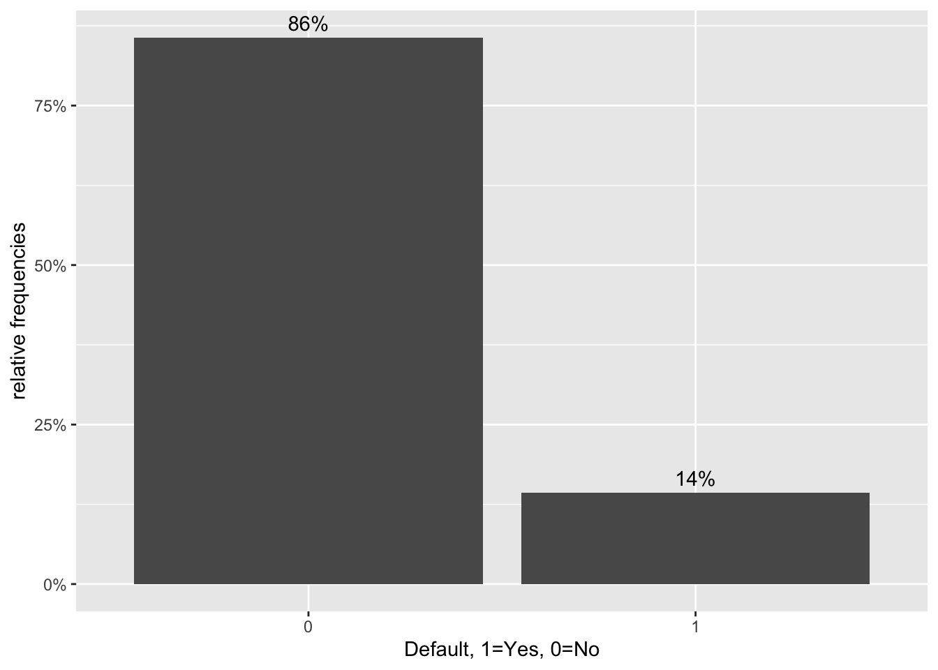

#bar chart of defaults per loan grade
def_vis2<-ggplot(data=lc_clean, aes(x=default), group=grade) +geom_bar(aes(y = (..count..)/sum(..count..), fill = factor(..x..)), stat="count")  + labs(title="Defaults by Grade", x="Default, 1=Yes, 0=No", y="relative frequencies") +scale_y_continuous(labels=scales::percent) +facet_grid(~grade) + theme(legend.position = "none") +geom_text(aes( label = scales::percent((..count..)/sum(..count..) ),y=(..count..)/sum(..count..) ), stat= "count",vjust=-0.5) 
def_vis2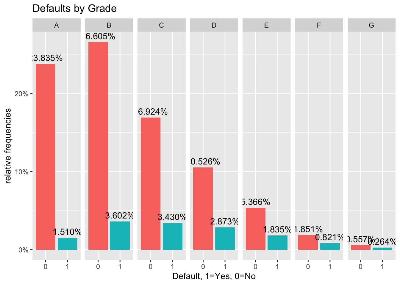

#bar chart of defaults per number of Delinquencies
def_vis3<-lc_clean %>%
  filter(as.numeric(delinq_2yrs)<4) %>%
  ggplot(aes(x=default), group=delinq_2yrs) +geom_bar(aes(y = (..count..)/sum(..count..), fill = factor(..x..)), stat="count")  + labs(title="Defaults by Number of Delinquencies", x="Default, 1=Yes, 0=No", y="relative frequencies")  +scale_y_continuous(labels=scales::percent) +facet_grid(~delinq_2yrs) + theme(legend.position = "none") +geom_text(aes( label = scales::percent((..count..)/sum(..count..) ),y=(..count..)/sum(..count..) ), stat= "count",vjust=-0.5)

def_vis3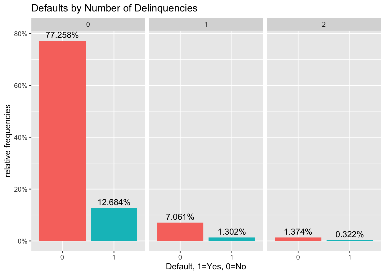

#scatter plots 

#We select 2000 random loans to display only to make the display less busy. 
set.seed(1234)
reduced<-lc_clean[sample(0:nrow(lc_clean), 2000, replace = FALSE),]%>%
  mutate(default=as.numeric(default)-1) # also convert default to a numeric {0,1} to make it easier to plot.

          
# scatter plot of defaults against loan amount                         
def_vis4<-ggplot(data=reduced, aes(y=default,x=I(loan_amnt/1000)))  + labs(y="Default, 1=Yes, 0=No", x="Loan Amnt (1000 $)") +geom_jitter(width=0, height=0.05, alpha=0.7) #We use jitter to offset the display of defaults/non-defaults to make the data easier to interpert. We have also changed the amount to 1000$ to reduce the number of zeros on the horizontal axis.

def_vis4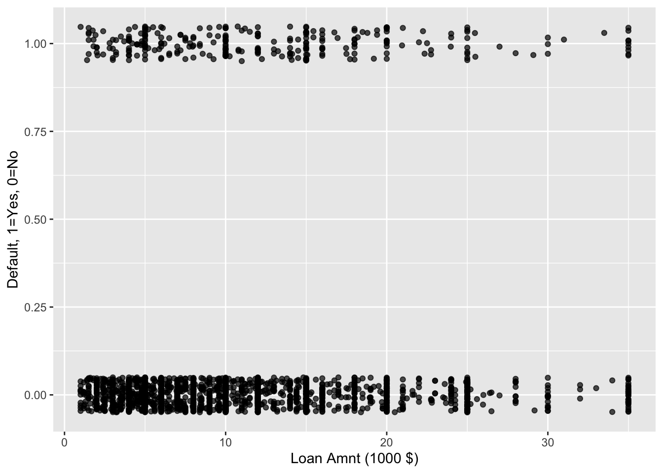

#scatter plot of defaults against loan amount.
def_vis5<-ggplot(data=reduced, aes(y=default,x=I(annual_inc/1000)))   + labs(y="Default, 1=Yes, 0=No", x="Annual Income(1000 $)") +geom_jitter(width=0, height=0.05, alpha=0.7) +  xlim(0,400)

def_vis5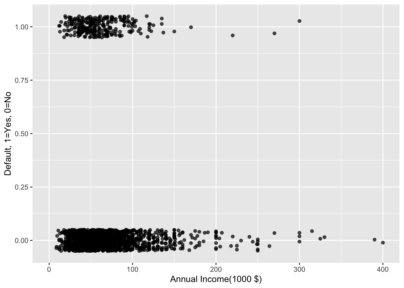

We can also estimate a correlation table between defaults and other continuous variables.

# correlation table using GGally::ggcor()
# this takes a while to plot

lc_clean %>% 
    mutate(default=as.numeric(default)-1) %>%
  select(loan_amnt, dti, annual_inc, int_rate, default) %>% #keep Y variable last
 ggcorr(method = c("pairwise", "pearson"), label_round=2, label = TRUE)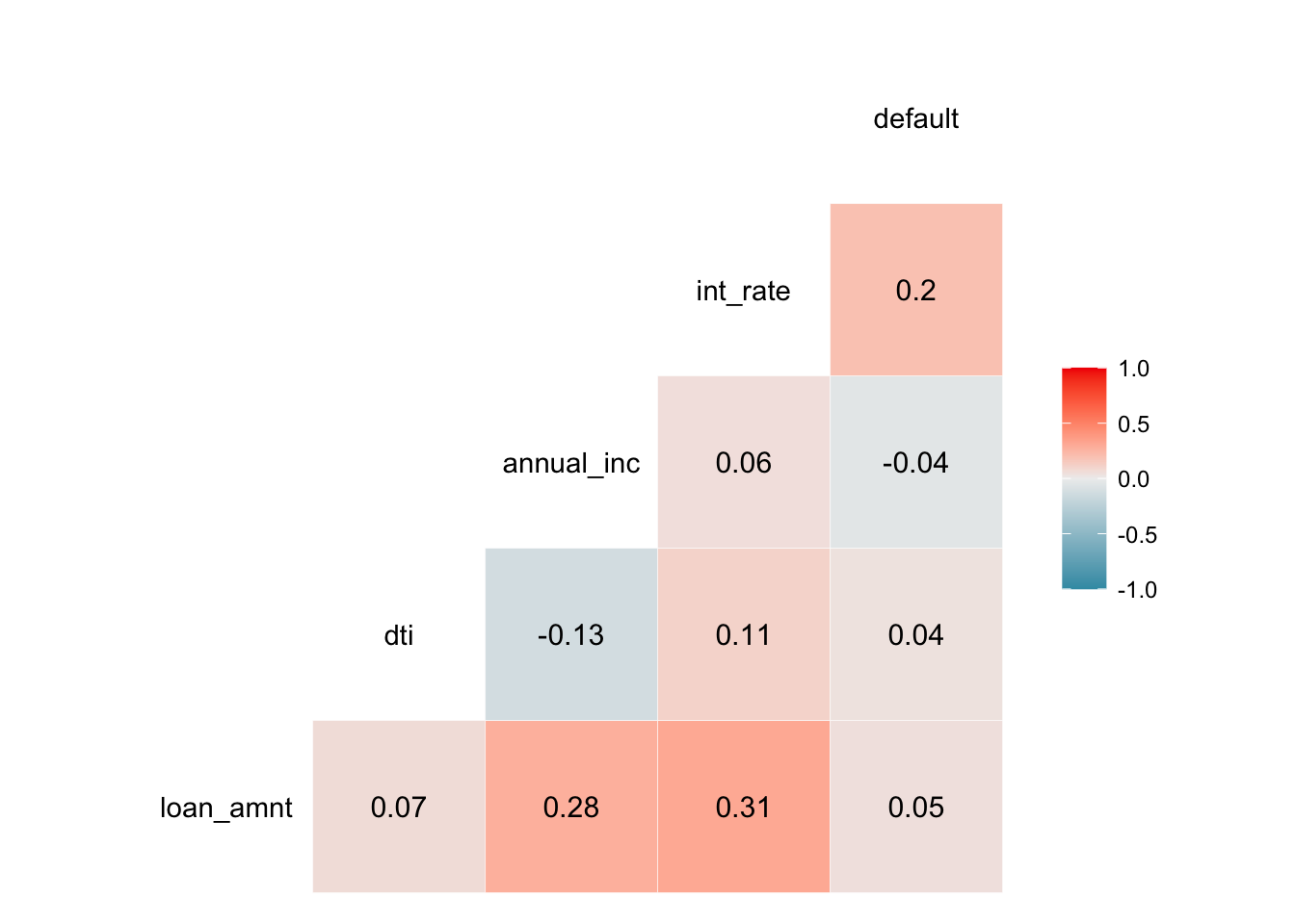

#bar chart of defaults per number of term months
def_vis6<-lc_clean %>%
  ggplot(aes(x=default), group=term) +
  geom_bar(aes(y = (..count..)/sum(..count..), fill = factor(..x..)), stat="count")  + 
  labs(title="Defaults by Loan Term Months", 
       x="Default, 1=Yes, 0=No", 
       y="relative frequencies")  +
  scale_y_continuous(labels=scales::percent,limits=c(0,0.7)) +
  facet_grid(~term) + 
  theme(legend.position = "none") +
  geom_text(aes( label = scales::percent((..count..)/sum(..count..) ),y=(..count..)/sum(..count..) ), 
            stat= "count",vjust=-0.5)

def_vis6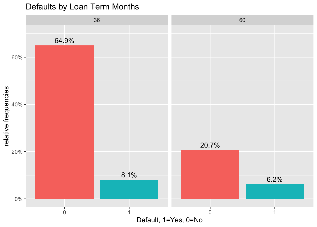

Comment: The graph above shows the relative frequencies of defaulted and not-defaulted loans compared by a loan term of 36 months vs. 60 months. We can see that there are more 36-months loans overall but, comparing default vs. no default per individual term length, we find that the share of loans that do not default compared to the share of loans that do default is greater for a loan term of 36 months than a loan of 60 months. Alternatively, a relatively greater share of 60-months loans defaults compared to a smaller proportion of 36 months that defaults.

Linear vs. logistic regression for binary response variables

It is certainly possible to use the OLS approach to find the line that minimizes the sum of square errors when the dependent variable is binary (i.e., default no default). In this case, the predicted values take the interpretation of a probability. We can also estimate a logistic regression instead. We do both below.

model_lm<-lm(as.numeric(default)~I(annual_inc/1000), lc_clean)
summary(model_lm)

## 
## Call:
## lm(formula = as.numeric(default) ~ I(annual_inc/1000), data = lc_clean)
## 
## Residuals:
##     Min      1Q  Median      3Q     Max 
## -0.1595 -0.1494 -0.1444 -0.1332  1.3268 
## 
## Coefficients:
##                      Estimate Std. Error t value Pr(>|t|)    
## (Intercept)         1.161e+00  2.703e-03 429.312   <2e-16 ***
## I(annual_inc/1000) -2.479e-04  2.918e-05  -8.496   <2e-16 ***
## ---
## Signif. codes:  0 '***' 0.001 '**' 0.01 '*' 0.05 '.' 0.1 ' ' 1
## 
## Residual standard error: 0.3501 on 37867 degrees of freedom
## Multiple R-squared:  0.001903,   Adjusted R-squared:  0.001876 
## F-statistic: 72.19 on 1 and 37867 DF,  p-value: < 2.2e-16

logistic1<-glm(default~I(annual_inc/1000), family="binomial", lc_clean)
summary(logistic1)

## 
## Call:
## glm(formula = default ~ I(annual_inc/1000), family = "binomial", 
##     data = lc_clean)
## 
## Deviance Residuals: 
##     Min       1Q   Median       3Q      Max  
## -0.6246  -0.5786  -0.5572  -0.5115   3.6388  
## 
## Coefficients:
##                      Estimate Std. Error z value Pr(>|z|)    
## (Intercept)        -1.5191545  0.0292430  -51.95   <2e-16 ***
## I(annual_inc/1000) -0.0040801  0.0003998  -10.21   <2e-16 ***
## ---
## Signif. codes:  0 '***' 0.001 '**' 0.01 '*' 0.05 '.' 0.1 ' ' 1
## 
## (Dispersion parameter for binomial family taken to be 1)
## 
##     Null deviance: 31130  on 37868  degrees of freedom
## Residual deviance: 31005  on 37867  degrees of freedom
## AIC: 31009
## 
## Number of Fisher Scoring iterations: 5

ggplot(data=reduced, aes(x=I(annual_inc/1000), y=default)) + geom_smooth(method="lm", se=0, aes(color="OLS"))+ geom_smooth(method = "glm", method.args = list(family = "binomial"),  se=0, aes(color="Logistic"))+ labs(y="Prob of Default", x="Annual Income(1000 $)")+  xlim(0,450)+scale_y_continuous(labels=scales::percent)+geom_jitter(width=0, height=0.05, alpha=0.7) + scale_colour_manual(name="Fitted Model", values=c("blue", "red"))

## `geom_smooth()` using formula 'y ~ x'
## `geom_smooth()` using formula 'y ~ x'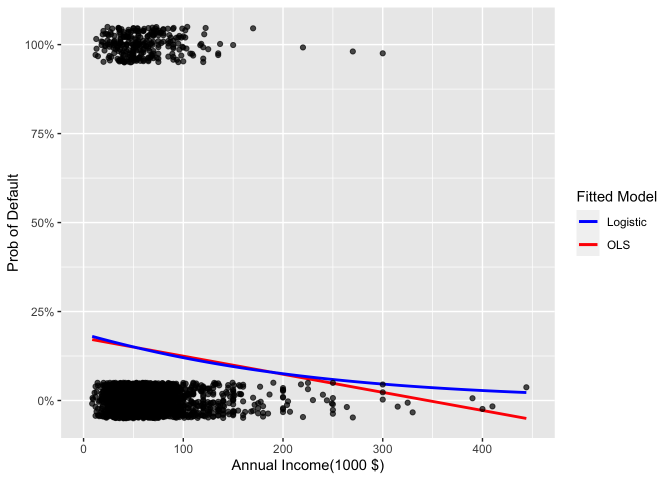

Which model is more suitable for predicting probability of default, the linear regression or the logistic? Why?

As the measure of fit for the linear regression is the R-squared (here 0.001903) but the measure of fit for the logistic regression is the Deviance (here 31005), we cannot compare these models along the lines of their measures of fit.

However, as the goal is to predict a probability of default, the logistic regression is more suitable for prediction regardless of the measure of fit. As we are predicting the probability of the binary variable default, we are predicting if default is 1 or 0. However, the OLS method does not take into account that, therefore, the only reasonable output is that the probability of a loan defaulting (default = 1) is (between) 0% and 100%. As can be seen in the graph above, the linear regression also predicts probabilities that are less than 0. Hence, the linear regression goes over the boundaries that are applicable for this prediction and we conclude that the logistic regression is more suitable here, as it limits the output probabilities at 0 and 1. This can be seen in the graph as the logistic model regression line does not go below 0 whereas the OLS regression line already does. According to the OLS regression, the loans of people with an annual income of more than approx $350,000 would have a negative probability of default - which is clearly not feasible in real life. The logistic model is limited at 0 and all probabilities of loan defaults for people with an annual income greater than $350k approach 0% but never become negative. Hence, the logistic regression is more suitable for predicting probability of default.

Multivariate logistic regression

We can estimate logistic regression with multiple explanatory variables as well. Let’s use annual_inc, term, grade, and loan amount as features. Let’s call this model logistic 2.

logistic2 <- glm(default ~ annual_inc + term + grade + loan_amnt, family = "binomial", lc_clean)
summary(logistic2)

## 
## Call:
## glm(formula = default ~ annual_inc + term + grade + loan_amnt, 
##     family = "binomial", data = lc_clean)
## 
## Deviance Residuals: 
##     Min       1Q   Median       3Q      Max  
## -1.0635  -0.6079  -0.4815  -0.3455   4.0988  
## 
## Coefficients:
##               Estimate Std. Error z value Pr(>|z|)    
## (Intercept) -2.432e+00  5.056e-02 -48.093   <2e-16 ***
## annual_inc  -6.019e-06  4.727e-07 -12.733   <2e-16 ***
## term60       4.790e-01  3.561e-02  13.451   <2e-16 ***
## gradeB       6.599e-01  5.270e-02  12.521   <2e-16 ***
## gradeC       1.031e+00  5.392e-02  19.128   <2e-16 ***
## gradeD       1.288e+00  5.703e-02  22.578   <2e-16 ***
## gradeE       1.415e+00  6.662e-02  21.241   <2e-16 ***
## gradeF       1.666e+00  8.630e-02  19.302   <2e-16 ***
## gradeG       1.769e+00  1.340e-01  13.198   <2e-16 ***
## loan_amnt    2.841e-06  2.347e-06   1.211    0.226    
## ---
## Signif. codes:  0 '***' 0.001 '**' 0.01 '*' 0.05 '.' 0.1 ' ' 1
## 
## (Dispersion parameter for binomial family taken to be 1)
## 
##     Null deviance: 31130  on 37868  degrees of freedom
## Residual deviance: 29286  on 37859  degrees of freedom
## AIC: 29306
## 
## Number of Fisher Scoring iterations: 5

#compare the fit of logistic 1 and logistic 2
anova(logistic1,logistic2)

Resid. Df	Resid. Dev	Df	Deviance
3.79e+04	3.1e+04
3.79e+04	2.93e+04	8	1.72e+03

Based on logistic 2, we explain the following: a. Estimated Coefficients b. Standard error of coefficient c. p-value of coefficient d. Deviance e. AIC f. Null Deviance g. Is Logistic 2 a better model than logistic 1? Why or why not?

The estimated coefficients must be transformed to probabilities with the following formula: P=exp(x)/(1+exp(x)). This will generate a probability per estimated coefficient. This probability describes the additional probability of increasing the respective coefficient’s unit by 1 that will be added to the predicted probability of the loan defaulting. For example, the term60 estimated coefficient is 4.790e-01; its probability is hence P = exp(0.479)/(1+exp(0.479)) = 0.6175117. This means that, compared to a 36-months loan, a 60-months loan has a 0.62 higher probability of default.
The Standard Error of each coefficient is an estimate of the standard deviation of the respective estimated coefficient; meaning, the amount the respective coefficient varies across cases. It measures the precision with which the respective coefficient is measured. For example, with a Std Error of 4.727e-07, annual_inc has the lowest estimated standard deviation of all coefficient estimates.
The p-value of each estimated coefficient determines the probability of extreme results as it tests the null hypothesis that the respective variable has no correlation with the dependent variable, namely here, that the respective variable has no correlation with a loan’s default. A variable is seen as statistically significant for a p-value below 5% (0.05). In the logistic2 model, we find that all variables except for loan_amnt are statistically significant (p-value < 0.05). As the p-value of loan_amnt is 0.226 >> 0.05, this coefficient is regarded as not significant in our logistic2 model.
We assess the in-sample goodness of fit of logistic regression with the Deviance (compared to the R-squared in linear regression). The lower the deviance, the better. R calculates: Deviance = -2log(L) where L is the maximum likelihood. Hence, the deviance is the difference of the likelihoods between the fitted model and a perfect model (=saturated model). The likelihood of the saturated/perfect model is exactly one, hence, the deviance is always larger than or equal to 0; being 0 if the fit is perfect. As part of the model summary(), R reports the deviance of the estimated model with all the specified features as well as the Null Deviance of the model with only the intercept as a comparison (assuming no explanatory variables). Here, the Null Deviance is 31130 while the Residual Deviance of our logistic2 model is lower at 29286. This means that logistic2 model with annual_inc, term, grade, and loan amount as predictors improves fit over the null model which does not have any predictors.
The AIC (Akaike Information Criterion) is similar to the Deviance as it assesses a model’s goodness of fit but it penalizes for the number of coefficients used in the model. In logistic regression, the AIC is to the Deviance what the adjusted R-squared is to the R-squared in linear regression. Its formula is: AIC = -2log(L) + 2k where k is the number of estimated coefficients. It is useful to compare different models with different numbers of features estimated on the same dataset. The Deviance of logistic 2 is 29286 and the AIC is relatively similar at 29306; considering that we use 4 features in our model, the AIC is more meaningful to assess the models goodness-of-fit.
Th Null Deviance is used as a benchmark to evaluate the magnitude of the Residual Deviance. It is the deviance of the worst model (a model fitted without any predictors) compared to the perfect/saturated model. The Null Deviance helps to understand how much a model improves by adding predictors. Here, the Null Deviance is 31130 and the Residual Deviance is 29286, indicating that adding our explanatory variables as part of logistic2 improves (reduces) the deviance of the model compared to the Null Deviance significantly.
logistic1 has a deviance of 31005 and logistic 2 has a deviance of 29286 as well as an AIC of 29306. Since when comparing different models with a different number of features, we consider their Deviance, we conclude that logistic2 is better than logistic1 because its Deviance is lower than that of logistic1.

We calculate the predicted probabilities associated with logistic 2 and plot them as a density chart. We also plot the density of the predictions for those loans that did default, and for the loans that did not.

#Predict the probability of default
prob_default2<-predict(logistic2,lc_clean, type="response")

#plot 1: Density of predictions
ggplot(lc_clean, aes(x=prob_default2))+  
  geom_density(size =0.75)+
  labs(title = "Predicted Probability with logistic2",
       x = "Estimated Probability",
       y = "Density")+
  NULL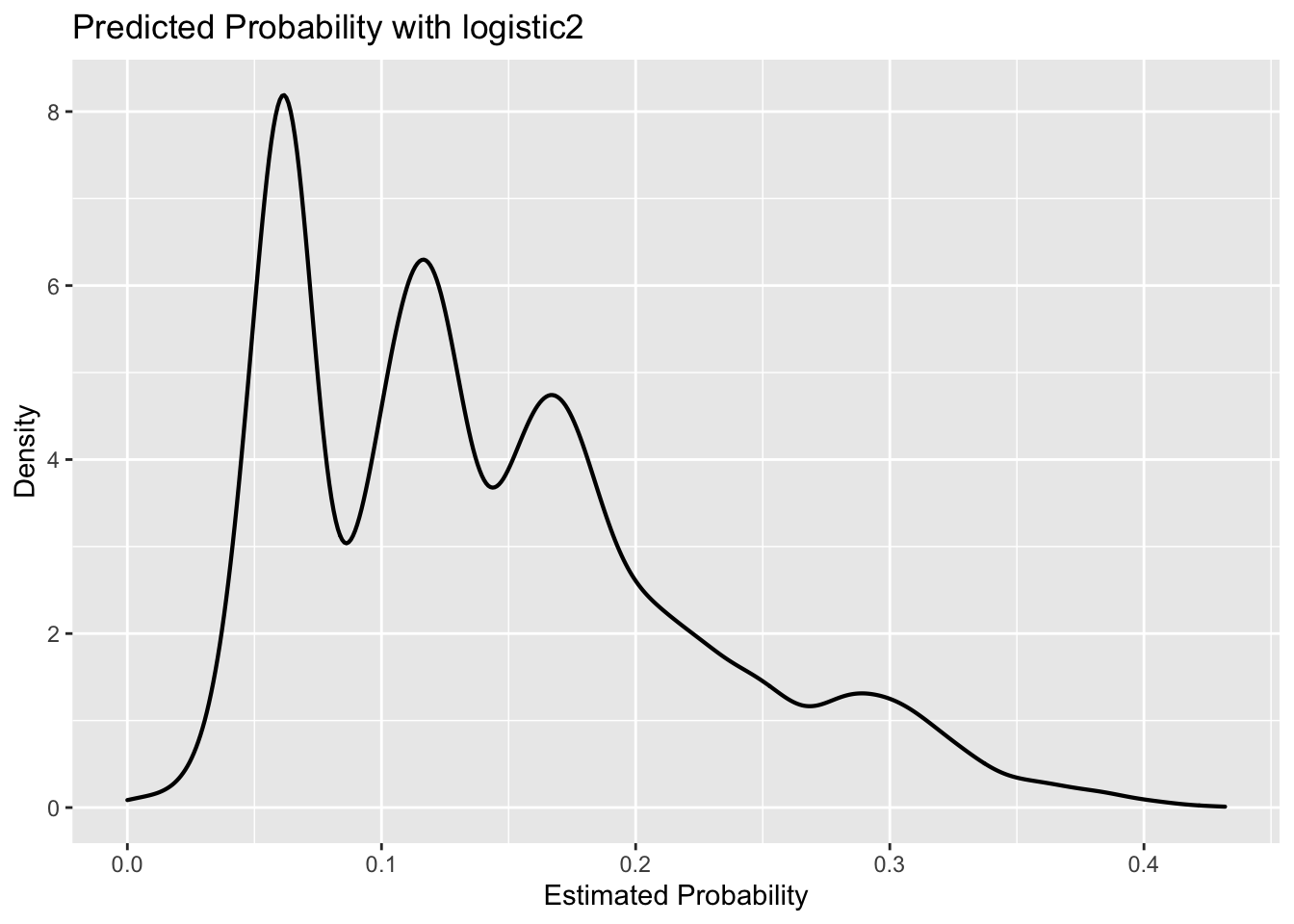

#plot 2: Density of predictions by default
ggplot(lc_clean, aes(x=prob_default2, colour = default))+  
  geom_density(size =0.75)+
  labs(title = "Predicted Probability by default with logistic2",
       x = "Estimated Probability",
       y = "Density",
       colour = "Default: \nNo = 0,\nYes = 1")+
  NULL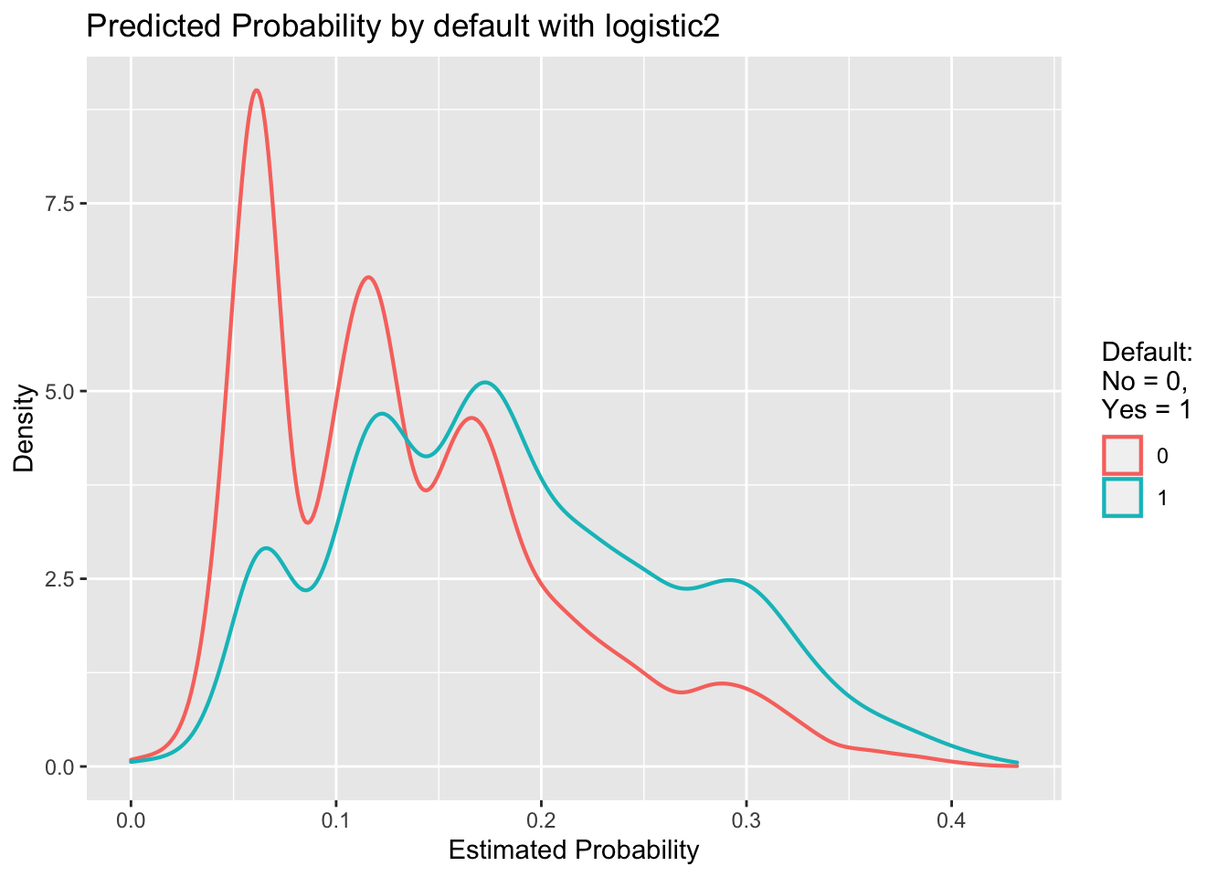

In the first plot, we see that the odds are the highest for a predicted default probability of approx. 0.06. We can also see that an estimated probability of approx. 0.125 (second peak) is approx. 6.2/8.1 = ~77% less likely.

Looking at the predicted probabilities by default (second graph) gives a better understanding of the differences between the defaulted and the non-defaulted loans as we see that the density curves do not follow the same trend and have different peaks, meaning different odds for different estimated probabilities of occurrence. While the peak of the non-defaulted loans density curve is at an estimated probability of approx. 0.06, the peak of the defaulted loans density curve is at approx. 0.175.

Since the two density plots overlap, we know that there will be a sharp trade-off between sensitivity and specificity of the outcomes. This means that it is difficult (up to impossible) to avoid situations in which we make many mistakes (either predicting a loan to default when it actually does not default or predicting a loan to not default when it actually does default). Had the two density curves not/hardly overlapped, we would’ve been more likely to make fewer mistakes while, at the same time, it would have been easier for us to determine a cut-off threshold (see next exercise).

From probability to classification

The logistic regression model gives us a sense of how likely defaults are; it gives us a probability estimate. To convert this into a prediction, we need to choose a cutoff probability and classify every loan with a predicted probability of default above the cutoff as a prediction of default (and vice versa for loans with a predicted probability below this cutoff).

Let’s choose a threshold of 20%. Of course some of our predictions will turn out to be right but some will turn out to be wrong – we can see this in the density figures of the previous section. Let’s call “default” the “positive” class since this is the class we are trying to predict. We could be making two types of mistakes. False positives (i.e., predict that a loan will default when it will not) and false negatives (I.e., predict that a loan will not default when it does). These errors are summarized in the confusion matrix.

We Produce the confusion matrix for the model logistic 2 for a cutoff of 18%

#using the logistic 2 model predict default probabilities
#already defined in code chunk above

#prob_default2<-predict(logistic2,lc_clean, type="response")
  
#Call any loan with probability more than 18% as default and any loan with lower probability as non-default. Making sure our prediction is a factor with the same levels as the default variable in the lc_clean data frame

#if probability is greater than cutoff 18%, then output is 1, otherwise output is 0
one_or_zero <- ifelse(prob_default2 > 0.18,"1","0")

#class prediction (vector of predictions of default (1) vs. non-default (0))
p_class <- factor(one_or_zero, levels = levels(lc_clean$default))
  
#produce the confusion matrix and set default as the positive outcome (i.e. consider outcome default as positive)
conmat <- confusionMatrix(p_class, lc_clean$default, positive = "1")

#print the confusion matrix
conmat

## Confusion Matrix and Statistics
## 
##           Reference
## Prediction     0     1
##          0 24674  2818
##          1  7766  2611
##                                         
##                Accuracy : 0.7205        
##                  95% CI : (0.716, 0.725)
##     No Information Rate : 0.8566        
##     P-Value [Acc > NIR] : 1             
##                                         
##                   Kappa : 0.1751        
##                                         
##  Mcnemar's Test P-Value : <2e-16        
##                                         
##             Sensitivity : 0.48094       
##             Specificity : 0.76060       
##          Pos Pred Value : 0.25161       
##          Neg Pred Value : 0.89750       
##              Prevalence : 0.14336       
##          Detection Rate : 0.06895       
##    Detection Prevalence : 0.27402       
##       Balanced Accuracy : 0.62077       
##                                         
##        'Positive' Class : 1             
##

Using the confusion matrix, we explain the following and show how they are calculated a. Accuracy b. Sensitivity c. Specificity For each of this, we explain what they mean in the context of the lending club and the goal of predicting loan defaults.

Answer:

Accuracy = 0.7205. This is the probability that a prediction will be correct (given by number of true predictions divided by the total number of predictions). Here, the probability that a default is truly predicted as a default or a non-default is truly predicted as a non-default is 72.05%. This is calculated by (sum of defaults correctly predicted as defaults + sum of non-defaults correctly predicted as non-defaults)/(total number of all predictions).
Sensitivity = 0.48094. This tells us how often positive outcomes (i.e., defaults) are predicted correctly (also referred to as true positive rate). Here, the probability that a default is correctly predicted as a default is ~48.1%. This is calculated by (sum of defaults correctly predicted as defaults)/(total number of all default predictions).
Specificity = 0.76060. This tells us how often negative outcomes (i.e., non-defaults) are predicted correctly (also referred to as true negative rate). Here, the probability that a non-default is correctly predicted as a non-default is ~76.1%. This is calculated by (sum of non-defaults correctly predicted as non-defaults)/(total number of all non-default predictions).

Using the model logistic 2, we produce the ROC curve and calculate the AUC measure. We xplain what the ROC shows and what the AUC measure means. Why do we expect the AUC of any predictive model to be between 0.5 and 1? Could the AUC ever be below 0.5 or above 1?

#estimate the ROC curve for Logistic 2
ROC_logistic2 <- roc(lc_clean$default, prob_default2)

## Setting levels: control = 0, case = 1

## Setting direction: controls < cases

#estimate the AUC for Logistic 2 and round it to two decimal places
AUC2<-round(auc(lc_clean$default,prob_default2)*100, digits=2)

## Setting levels: control = 0, case = 1
## Setting direction: controls < cases

#Plot the ROC curve and display the AUC in the title
ROC2 <- ggroc(ROC_logistic2,  alpha = 0.5) + 
  ggtitle(paste("Model Logistic 2: AUC=", AUC2, "%")) +
  geom_segment(aes(x = 1, xend = 0, y = 0, yend = 1), color="grey", linetype="dashed") +
  geom_segment(aes(x = 1, xend = 1, y = 0, yend = 1), color="black", linetype="dashed") +
  geom_segment(aes(x = 1, xend = 0, y = 1, yend = 1), color="black", linetype="dashed") +
  NULL

ROC2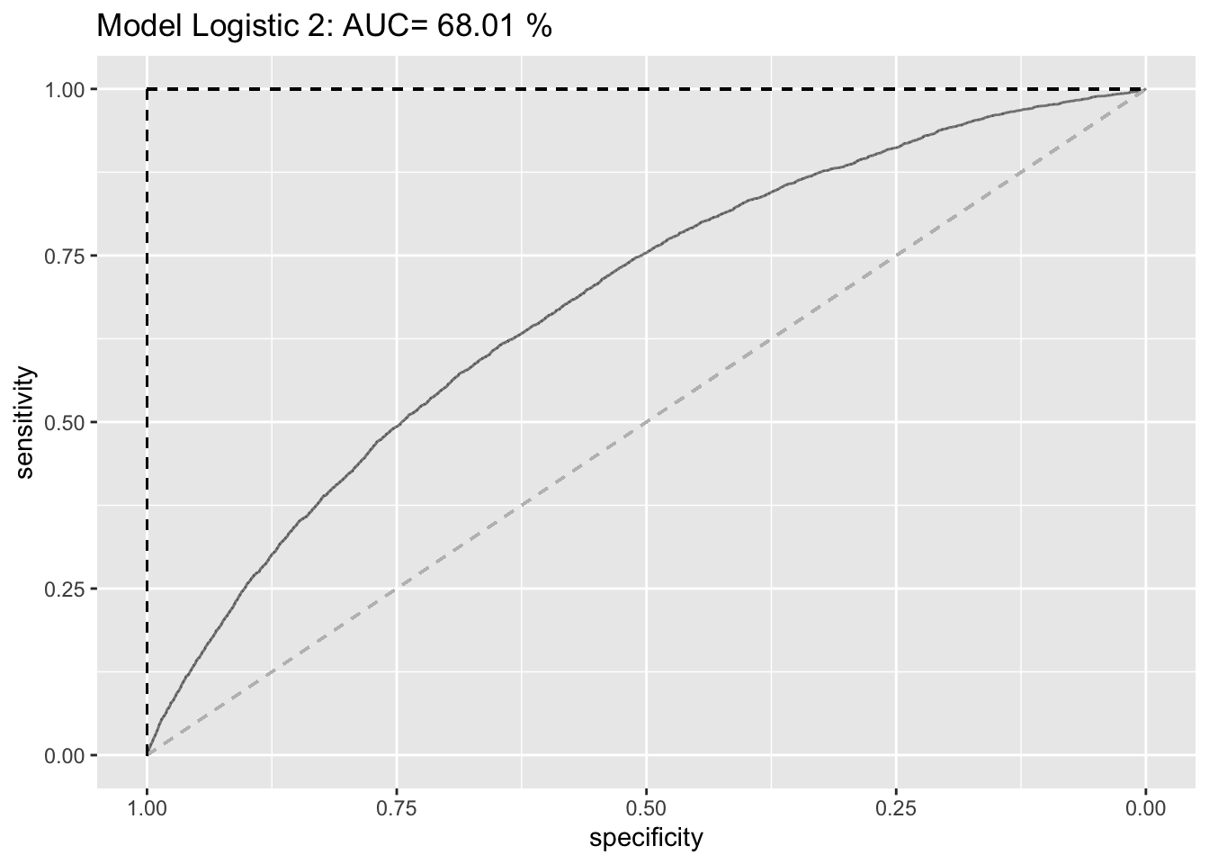

ROC and AUC are crucial evaluation metrics for the performance of any classification model. The ROC curve is another way to assess model performance that is agnostic to the cost of classification errors; it can help us in deciding which threshold value to choose. It does this by plotting the specificity against the respective sensitivity of all cutoff rates between 0 and 1. AUC means Area under the curve and gives the rate of successful classification by our logistic model. While the AUC is a helpful summary statistic of how well a model explains the data, it also helps in comparing ROC curves of models with each other. The higher the AUC per curve, the better; meaning, the better the model did at classification.

The gray dashed line describes a model that is not better than chance (i.e. a random classifier) in which the ROC curve would be a straight line from (1,0) to (0,1) with an AUC (area under the curve) of 0.5 (50%). The black dashed line, on the other hand, describes a perfect classifier in which all predictions are 100% correct and, therefore, both specificity as well as sensitivity would be 100%. The AUC, here, would be 1 (100%). Usually, the AUC is, therefore, between 0.5 and 1 as a useful model should perform better than random but could never perform better than getting 100% right - it could never be above 1. Theoretically, however, the AUC could also be below 0.5. This would mean that the classifier performs even worse than a random classifier and, thereby, indicate an non-useful model. Usually, this indicates that something went wrong or that we were particularly unlucky with our data split into train and test sets in a way that the patterns that are supposed to be classified are systematically different.

To sum up, the AUC values always lie between 0 and 1; meaning, the AUC can be below 0.5 but not above 1 (and not below 0). We do however expect it to be greater than 0.5 as a useful model should perform better than random chance. This indicates a constant trade-off between sensitivity and specificity. Above, we can see that our logistic2 model is better than a random classifier but not as good as the perfect classifier with an AUC of 68.01%.

So far we have only worked in-sample. We, now, split the data into training and testing and estimate the models ROC curve and AUC measure out of sample. Is there any evidence of over fitting?

# splitting the data into training and testing
set.seed(1234)
train_test_split <- initial_split(lc_clean, prop = 0.8)
testing <- testing(train_test_split) #20% of the data is set aside for testing
training <- training(train_test_split) #80% of the data is set aside for training

# run logistic 2 on the training set 
logistic2_train <- glm(default ~ annual_inc + term + grade + loan_amnt, family= "binomial", training)

## Warning: glm.fit: fitted probabilities numerically 0 or 1 occurred

#calculate probability of default in the training sample 
p_in <- predict(logistic2_train, training, type = "response") 

#ROC curve using in-sample predictions
ROC_logistic2_in <- roc(training$default, p_in)

## Setting levels: control = 0, case = 1

## Setting direction: controls < cases

#AUC using in-sample predictions
AUC_logistic2_in <- round(auc(training$default, p_in)*100, digits=2)

## Setting levels: control = 0, case = 1
## Setting direction: controls < cases

#calculate probability of default out of sample 
p_out <- predict(logistic2_train, testing, type = "response") 

#ROC curve using out-of-sample predictions
ROC_logistic2_out <- roc(testing$default, p_out)

## Setting levels: control = 0, case = 1
## Setting direction: controls < cases

#AUC using out-of-sample predictions
AUC_logistic2_out <- round(auc(testing$default, p_out)*100, digits=2)

## Setting levels: control = 0, case = 1
## Setting direction: controls < cases

#plot in the same figure both ROC curves and print the AUC of both curves in the title
ROC_both <- ggroc(list("Logistic 2 in-sample"=ROC_logistic2_in, "Logistic 2 out-of-sample"=ROC_logistic2_out)) +
  ggtitle(paste("Model Logistic 2 in-sample AUC=", 
                AUC_logistic2_in,"%\nModel Logistic 2 out-of-sample AUC=",
                AUC_logistic2_out,"%"))+
  geom_segment(aes(x = 1, xend = 0, y = 0, yend = 1), color="grey", linetype="dashed")+
  geom_segment(aes(x = 1, xend = 1, y = 0, yend = 1), color="black", linetype="dashed") +
  geom_segment(aes(x = 1, xend = 0, y = 1, yend = 1), color="black", linetype="dashed") +
  labs(colour = "ROC curves") +
  NULL

ROC_both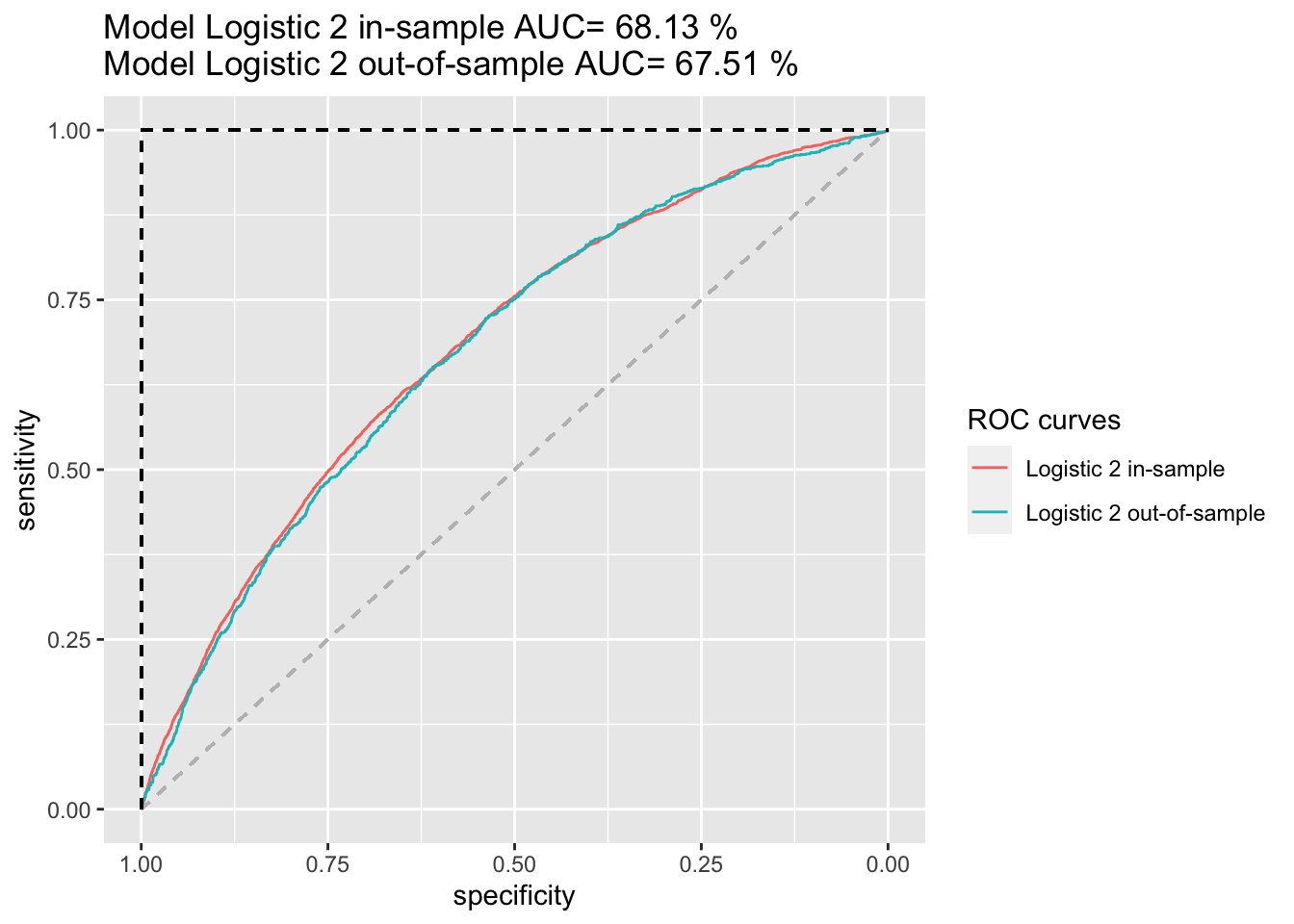

Above, we can see that the in-sample and the out-of-sample logistic2 ROC curves are very similar and both have a similar AUC of 68.13% and 67.51% respectively. These results are subject to the set seed and, thereby, how the data is divided between testing and training set.

We cannot use the training set (in-sample) by itself to evaluate overfitting as it cannot measure the logistic2 model’s generalization performance. However, comparing the ROC curves of the training and testing set, namely the size of the gap between both, can help us to investigate overfitting. A large gap between the training and testing metrics indicates overfitting, whereas no gap indicates underfitting; a good model should always produce a small gap. While it is difficult to make a precise judgement, we can see small gaps between the in-sample and out-of-sample ROC curves as well as a small difference of both AUCs and can, therefore, conclude that our logistic2 model does not suffer from overfitting but is a rather good fit/model.

Selecting loans to invest using the model Logistic 2.

Before we look for a better model than logistic 2 let’s see how we can use this model to select loans to invest. Let’s make the simplistic assumption that every loan generates $20 profit if it is paid off and $100 loss if it is charged off for an investor. Let’s use a cut-off value to determine which loans to invest in, that is, if the predicted probability of default for a loan is below this value then we invest in that loan and not if it is above.

To do this we split the data in three parts: training, validation, and testing.

# splitting the data into training and testing
set.seed(1234)
train_test_split <- initial_split(lc_clean, prop = 0.6)
training <- training(train_test_split) #60% of the data is set aside for training
remaining <- testing(train_test_split) #40% of the data is set aside for validation & testing
set.seed(4321)
train_test_split <- initial_split(remaining, prop = 0.5)
validation<-training(train_test_split) #50% of the remaining data (20% of total data) will be used for validation
testing<-testing(train_test_split) #50% of the remaining data (20% of total data) will be used for testing

We train logistic 2 on the training set above. We use the trained model to determine the optimal cut-off threshold based on the validation test. What is the optimal cutoff threshold? How much profit does it generate? Using the testing set, what is the profit per loan associated with the cutoff?

#train logistic2 on the training set
logistic2_train <- glm(default ~ annual_inc + term + grade + loan_amnt, family="binomial", training)

## Warning: glm.fit: fitted probabilities numerically 0 or 1 occurred

#predict probability of default on the validation set
p_val <- predict(logistic2_train, validation, type = "response") 

#we select the cutoff threshold using the estimated model and the validation set
#define profit and threshold
profit=0 
threshold=0
#loop over 100 thresholds
for(i in 1:100) {
  threshold[i] = i/400  
  one_or_zero_search <- ifelse(p_val > threshold[i],"1","0")
  p_class_search <- factor(one_or_zero_search, levels = levels(validation$default))
  con_search <- confusionMatrix(p_class_search, validation$default, positive="1")
  #calculate profit according to the threshold
  profit[i] = con_search$table[1,1] * 20 -con_search$table[1,2] *100}

#plot profit against threshold
ggplot(as.data.frame(threshold), aes(x=threshold, y=profit)) + 
  geom_smooth(method = 'loess', se = 0) +
  labs(title = "Profit curve with logistic2 (based on the validation set)",
       x = "Cutoff threshold",
       y = "Profit") +
  NULL

## `geom_smooth()` using formula 'y ~ x'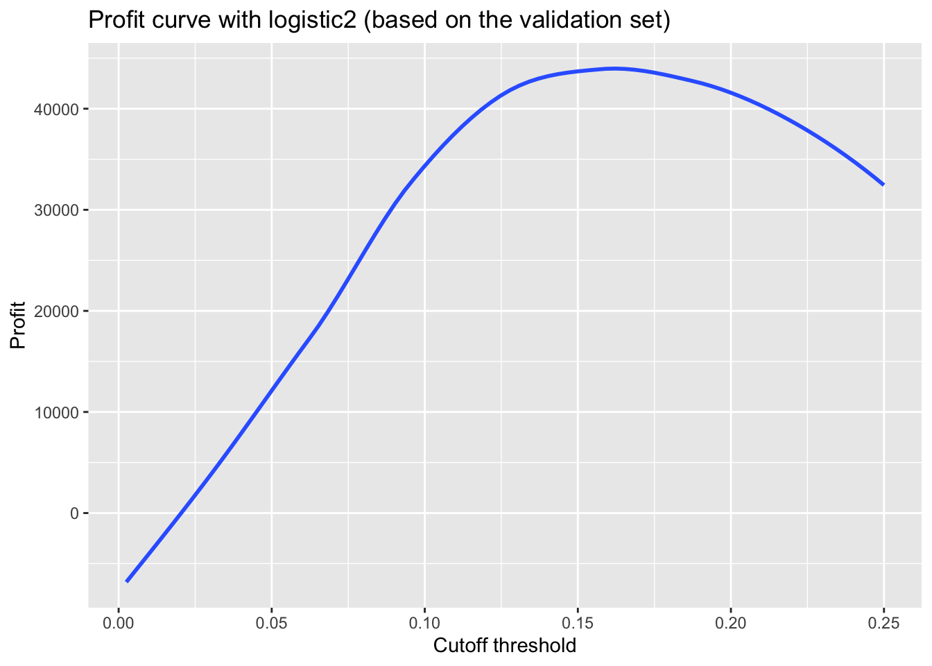

#output the maximum profit and the associated threshold based on the validation set
paste0("Based on the validation set, maximum profit per loan is $", round(max(profit) / nrow(validation), 2), " achieved at a cutoff threshold of ", threshold[which.is.max(profit)] * 100, "%.")

## [1] "Based on the validation set, maximum profit per loan is $5.92 achieved at a cutoff threshold of 15.5%."

#optimal threshold based on the validation set
threshold = threshold[which.is.max(profit)]
threshold

## [1] 0.155

#Using the model estimated on the training set above to predict probabilities of default on the testing set
#predict probability of default on the testing set
p_test<-predict(logistic2_train, testing, type = "response")

#use the threshold estimated using the validation set to estimate the profits on the testing set
one_or_zero <- ifelse(p_test>threshold,"1","0")
p_class <- factor(one_or_zero, levels = levels(testing$default))
con_test <- confusionMatrix(p_class, testing$default, positive = "1")
profit = con_test$table[1,1] * 20 - con_test$table[1,2] * 100
paste0("Based on the testing set, the profit per loan associated with a cuttoff threshold of ", threshold*100, "% is: $", round(profit/nrow(testing),2))

## [1] "Based on the testing set, the profit per loan associated with a cuttoff threshold of 15.5% is: $5.4"

Above, we firstly trained logistic2 on the previously defined training set. Then, we used this trained model on the validation set and, thereby, determined the maximum profit per loan to be $5.92 achieved at a cutoff threshold of 15.5% (peak of the curve in the profit curve plot) based on the validation set. Lastly, we used the trained model on the testing set and, using the 15.5% optimal cutoff threshold, found the profit per loan to be $5.40.

More realistic revenue model

Let’s build a more realistic profit and loss model. Each loan has different terms (e.g., different interest rate and different duration) and therefore a different return if fully paid. For example, a 36 month loan of $5000 with installment of $163 per month would generate a return of 163*36/5000-1 if there was no default. Let’s assume that it would generate a loss of -60% if there was a default (the loss is not 100% because the loan may not default immediately and/or the lending club may be able to recover part of the loan).

Under these assumptions, how much return would we get if we invested $1 in each loan in the validation set?

#investment of $1 per loan in validation set 
invest <- validation %>% 
            count()

invest # = 7574 loans meaning investment of $7574

n
7574

#calculate return per each loan in validation set for $1 investment in each loan
val_return <- validation %>%
  #create new return column
 mutate(return = 
          #if default per loan equals 0 / if loan did not default
          ifelse(default=="0",
                 #calculate return like this
                 (installment*term_months/loan_amnt -1),
                 #if loan did default, -60% (here -0.6 as this is -60% of $1)
                 -0.6))%>%
  summarize(
    #calculate total return
    total_return = sum(round(return,4)),
    #calculate return on investment in %
    return_on_invest = (round(total_return/as.numeric(invest)*100,5))
    )

val_return

total_return	return_on_invest
862	11.4

When investing $1 per loan in the validation set, we would invest a total of $7574 in all loans. According to the profit and loss dynamics, we would make a total return of ~$861.96 on these loans, meaning we would make a 11.38% return on investment (861.9565/7574*100).

Unfortunately, we cannot use the realized return to select loans to invest (as at the time we make the investment decision we do not know which loan will default). Instead, we can calculate an expected return using the estimated probabilities of default – expected return = return if not default * (1-prob(default)) + return if default * prob(default).

We calculate the expected return of the loans in the validation set using the logistic 2 model trained in the training set. Can we use the expected return metric to select a portfolio of the $n$ most promising loans to invest in ($n$ is an integer number)? How does the realized return vary as we change $n$? What is the profit for $n=800$?

#logistic2_train <- glm(default ~ annual_inc + term + grade + loan_amnt, family="binomial", training)
#p_val <- predict(logistic2_train, validation, type = "response")

validation_new <- cbind(validation, p_val)

returns <- validation_new %>% 
  mutate(
    #return if not default
    profit = installment*term_months/loan_amnt-1,
    #return if default
    loss = -0.6,
    #probability of not default
    profit_prob = 1-p_val,
    #probability of default
    loss_prob = p_val,
    #expected return
    expected_return = profit * profit_prob + loss * loss_prob,
    ) 

#select a portfolio of the n most promising loans to invest in
#we use the arrange function to sort by most promising loans to least promising loans
#use this code for any n

# returns %>% 
  # arrange(desc(expected_return)) %>% 
  # top_n(n) %>%
  # mutate(real_return = ifelse(default == "0", (installment*term_months/loan_amnt-1),-0.6)) %>%
  # summarize(
  # total_exp_return = sum(expected_return),
  # total_real_return = sum(real_return),
  # exp_return_on_invest = (total_exp_return/n*100),
  # real_return_on_invest = (total_real_return/n*100)
  # )

#for n = 600
returns %>% 
  arrange(desc(expected_return)) %>% 
  top_n(600) %>% 
  mutate(real_return = ifelse(default == "0", (installment*term_months/loan_amnt-1),-0.6)) %>%
  summarize(
  total_exp_return = sum(expected_return),
  total_real_return = sum(real_return),
  exp_return_on_invest = (total_exp_return/600*100),
  real_return_on_invest = (total_real_return/600*100)
  )

## Selecting by expected_return

total_exp_return	total_real_return	exp_return_on_invest	real_return_on_invest
149	150	24.8	24.9

  #total_exp_return = 149.0619  
  #total_real_return = 149.6932 
  #exp_return_on_invest = 24.84365  
  #real_return_on_invest = 24.94886 

#for n = 800
returns %>% 
  arrange(desc(expected_return)) %>% 
  top_n(800) %>% 
  mutate(real_return = ifelse(default == "0", (installment*term_months/loan_amnt-1),-0.6)) %>%
  summarize(
  total_exp_return = sum(expected_return),
  total_real_return = sum(real_return),
  exp_return_on_invest = (total_exp_return/800*100),
  real_return_on_invest = (total_real_return/800*100)
  )

## Selecting by expected_return

total_exp_return	total_real_return	exp_return_on_invest	real_return_on_invest
188	186	23.6	23.3

  #total_exp_return = 188.4074      
  #total_real_return = 186.4975 
  #exp_return_on_invest = 23.55093  
  #real_return_on_invest = 23.31219 

#for n = 1000
returns %>% 
  arrange(desc(expected_return)) %>% 
  top_n(1000) %>% 
  mutate(real_return = ifelse(default == "0", (installment*term_months/loan_amnt-1),-0.6)) %>%
  summarize(
  total_exp_return = sum(expected_return),
  total_real_return = sum(real_return),
  exp_return_on_invest = (total_exp_return/1000*100),
  real_return_on_invest = (total_real_return/1000*100)
  )

## Selecting by expected_return

total_exp_return	total_real_return	exp_return_on_invest	real_return_on_invest
225	213	22.5	21.3

  #total_exp_return = 225.4676  
  #total_real_return = 212.9639 
  #exp_return_on_invest = 22.54676
  #real_return_on_invest = 21.29639 

#for n = 5000
returns %>% 
  arrange(desc(expected_return)) %>% 
  top_n(5000) %>% 
  mutate(real_return = ifelse(default == "0", (installment*term_months/loan_amnt-1),-0.6)) %>%
  summarize(
  total_exp_return = sum(expected_return),
  total_real_return = sum(real_return),
  exp_return_on_invest = (total_exp_return/5000*100),
  real_return_on_invest = (total_real_return/5000*100)
  )

## Selecting by expected_return

total_exp_return	total_real_return	exp_return_on_invest	real_return_on_invest
693	680	13.9	13.6

  #total_exp_return = 692.7218  
  #total_real_return = 679.7163
  #exp_return_on_invest = 13.85444  
  #real_return_on_invest = 13.59433

#for n = 7574 (all)
returns %>% 
  arrange(desc(expected_return)) %>% 
  top_n(7547) %>% 
  mutate(real_return = ifelse(default == "0", (installment*term_months/loan_amnt-1),-0.6)) %>%
  summarize(
  total_exp_return = sum(expected_return),
  total_real_return = sum(real_return),
  exp_return_on_invest = (total_exp_return/7547*100),
  real_return_on_invest = (total_real_return/7547*100)
  )

## Selecting by expected_return

total_exp_return	total_real_return	exp_return_on_invest	real_return_on_invest
868	861	11.5	11.4

  #total_exp_return = 867.8876      
  #total_real_return = 860.5416 
  #exp_return_on_invest = 11.49977
  #real_return_on_invest = 11.40243

As can be seen above, inserting different values for n, shows us how the total expected return and the realized return as well as the expected and realized return on investment (in %) differ for different numbers n of the top most promising loans. Here, we arrange the expected returns in descending order to sort the data set by most promising loans to least promising loans. We find that the both the expected return as well as the realized return steadily increase with increasing n (up to a total return of ~$861.96 for all loans as we already calculated in the exercise before). The expected as well as the realized return on investment, however, decrease with increasing n. This is because we have an increasing number of loans (n) while, at the same time, the returns get increasingly smaller (since we sorted the data from highest to lowest expected return). Looking at the 800 most promising loans (n=800), we find the expected profit to be ~$188.41 (ROI of ~23.55%) and the realized profit to be ~$186.50 (ROI of ~23.31%).

For $n=800$, how sensitive is our answer to the assumption that if a loan defaults we lose 60% of the value? To answer this question, we assess how the realized return of the 800 loans chosen in our portfolio change if the loss proportion varies from 20%-80%?

#repeat above actions with loss of -20% instead of -60%
returns_check1 <- validation_new %>% 
  mutate(
    profit = installment*term_months/loan_amnt-1,
    #check for loss of -20%
    loss = -0.2,
    profit_prob = 1-p_val,
    loss_prob = p_val,
    expected_return = profit * profit_prob + loss * loss_prob,
    ) 

#for n = 800
returns_check1 %>% 
  arrange(desc(expected_return)) %>% 
  top_n(800) %>% 
  mutate(real_return = ifelse(default == "0", (installment*term_months/loan_amnt-1),-0.2)) %>%
  summarize(
  total_exp_return = sum(expected_return),
  total_real_return = sum(real_return),
  exp_return_on_invest = (total_exp_return/800*100),
  real_return_on_invest = (total_real_return/800*100)
  )

## Selecting by expected_return

total_exp_return	total_real_return	exp_return_on_invest	real_return_on_invest
265	261	33.2	32.6

  #total_exp_return = 265.2958  
  #total_real_return = 261.097  
  #exp_return_on_invest = 33.16197  
  #real_return_on_invest = 32.63712

#repeat above actions with loss of -80% instead of -60%
returns_check2 <- validation_new %>% 
  mutate(
    profit = installment*term_months/loan_amnt-1,
    #check for loss of -80%
    loss = -0.8,
    profit_prob = 1-p_val,
    loss_prob = p_val,
    expected_return = profit * profit_prob + loss * loss_prob,
    ) 

#for n = 800
returns_check2 %>% 
  arrange(desc(expected_return)) %>% 
  top_n(800) %>% 
  mutate(real_return = ifelse(default == "0", (installment*term_months/loan_amnt-1),-0.8)) %>%
  summarize(
  total_exp_return = sum(expected_return),
  total_real_return = sum(real_return),
  exp_return_on_invest = (total_exp_return/800*100),
  real_return_on_invest = (total_real_return/800*100)
  )

## Selecting by expected_return

total_exp_return	total_real_return	exp_return_on_invest	real_return_on_invest
155	146	19.4	18.2

  #total_exp_return = 155.1385          
  #total_real_return = 145.941  
  #exp_return_on_invest = 19.39231  
  #real_return_on_invest = 18.24263

Our answers are highly sensitive to the assumption that if a loan defaults, we lose 60% of the value. Testing the same calculations but replacing the -60% once with -20% and once with -80% shows us that the smaller the loss is (e.g. -20%), the higher the expected and realized return - this is logical as our total profit increases when we decrease individual losses. In addition to the higher return, the expected and realized returns on investment also increase with decreasing value loss. Vice versa, we find that increasing the proportional loss (e.g. here to 80%) will significantly decrease our returns as well as the relative returns on investment. More precisely, changing the value loss when a loan defaults from -20% to -60% to -80% decreases the expected (realized) return from $265.30 ($261.10) to $188.41 ($186.50) to $155.14 ($145.94) respectively. At the same time, the expected (realized) return on investment decreases from 33.16 (32.64) to 23.55% (23.31%) to 19.39% (18.24%) respectively.

Finally and to sum up, the realized return of the 800 most promising loans varies between $261.10 and $145.94 depending on the loss proportion varying between -20% and -80% respectively. This significant difference of ~$115 in realized return depending on the loss proportion indicates that our answers are highly sensitive to the specific loss proportion we assume.

We experiment with different models using more features, interactions, and non-linear transformations. We may also want to try to estimate models using regularization (e.g., LASSO regression) or use data from other sources (making sure our model does not use information that would not be available at the time the loan is extended (e.g., for a 4-year loan given in January 2008, we can’t use macro-economic indicators for 2008 or 2009 to predict whether the loan will default)). We present below our best model and explain why we have chosen it.

#final model
finalmodel <- glm(default ~ log(annual_inc) + loan_amnt:int_rate + term + log(int_rate):grade, family = "binomial", lc_clean)
summary(finalmodel)

## 
## Call:
## glm(formula = default ~ log(annual_inc) + loan_amnt:int_rate + 
##     term + log(int_rate):grade, family = "binomial", data = lc_clean)
## 
## Deviance Residuals: 
##     Min       1Q   Median       3Q      Max  
## -1.3077  -0.6034  -0.4693  -0.3275   2.7125  
## 
## Coefficients:
##                        Estimate Std. Error z value Pr(>|z|)    
## (Intercept)           6.499e+00  4.876e-01  13.328  < 2e-16 ***
## log(annual_inc)      -5.605e-01  3.124e-02 -17.943  < 2e-16 ***
## term60                4.470e-01  3.598e-02  12.423  < 2e-16 ***
## loan_amnt:int_rate    5.838e-05  1.571e-05   3.716 0.000203 ***
## log(int_rate):gradeA  1.236e+00  1.475e-01   8.380  < 2e-16 ***
## log(int_rate):gradeB  1.168e+00  1.720e-01   6.789 1.13e-11 ***
## log(int_rate):gradeC  1.107e+00  1.889e-01   5.858 4.69e-09 ***
## log(int_rate):gradeD  1.067e+00  2.037e-01   5.237 1.63e-07 ***
## log(int_rate):gradeE  1.075e+00  2.161e-01   4.977 6.46e-07 ***
## log(int_rate):gradeF  1.007e+00  2.313e-01   4.355 1.33e-05 ***
## log(int_rate):gradeG  1.010e+00  2.507e-01   4.027 5.64e-05 ***
## ---
## Signif. codes:  0 '***' 0.001 '**' 0.01 '*' 0.05 '.' 0.1 ' ' 1
## 
## (Dispersion parameter for binomial family taken to be 1)
## 
##     Null deviance: 31130  on 37868  degrees of freedom
## Residual deviance: 29100  on 37858  degrees of freedom
## AIC: 29122
## 
## Number of Fisher Scoring iterations: 5

#compare models
anova(logistic1, logistic2, finalmodel)

Resid. Df	Resid. Dev	Df	Deviance
3.79e+04	3.1e+04
3.79e+04	2.93e+04	8	1.72e+03
3.79e+04	2.91e+04	1	186

#plot ROC of final model
prob_default_fm<-predict(finalmodel,lc_clean, type="response")

ROC_logistic_fm <- roc(lc_clean$default, prob_default_fm)

## Setting levels: control = 0, case = 1

## Setting direction: controls < cases

#estimate the AUC for Logistic 2 and round it to two decimal places
AUC_fm<-round(auc(lc_clean$default,prob_default_fm)*100, digits=2)

## Setting levels: control = 0, case = 1
## Setting direction: controls < cases

#Plot the ROC curve and display the AUC in the title
ROC_fm <- ggroc(ROC_logistic_fm,  alpha = 0.5) + 
  ggtitle(paste("Final model: AUC=", AUC_fm, "%")) +
  geom_segment(aes(x = 1, xend = 0, y = 0, yend = 1), color="grey", linetype="dashed") +
  geom_segment(aes(x = 1, xend = 1, y = 0, yend = 1), color="black", linetype="dashed") +
  geom_segment(aes(x = 1, xend = 0, y = 1, yend = 1), color="black", linetype="dashed") +
  NULL

ROC_fm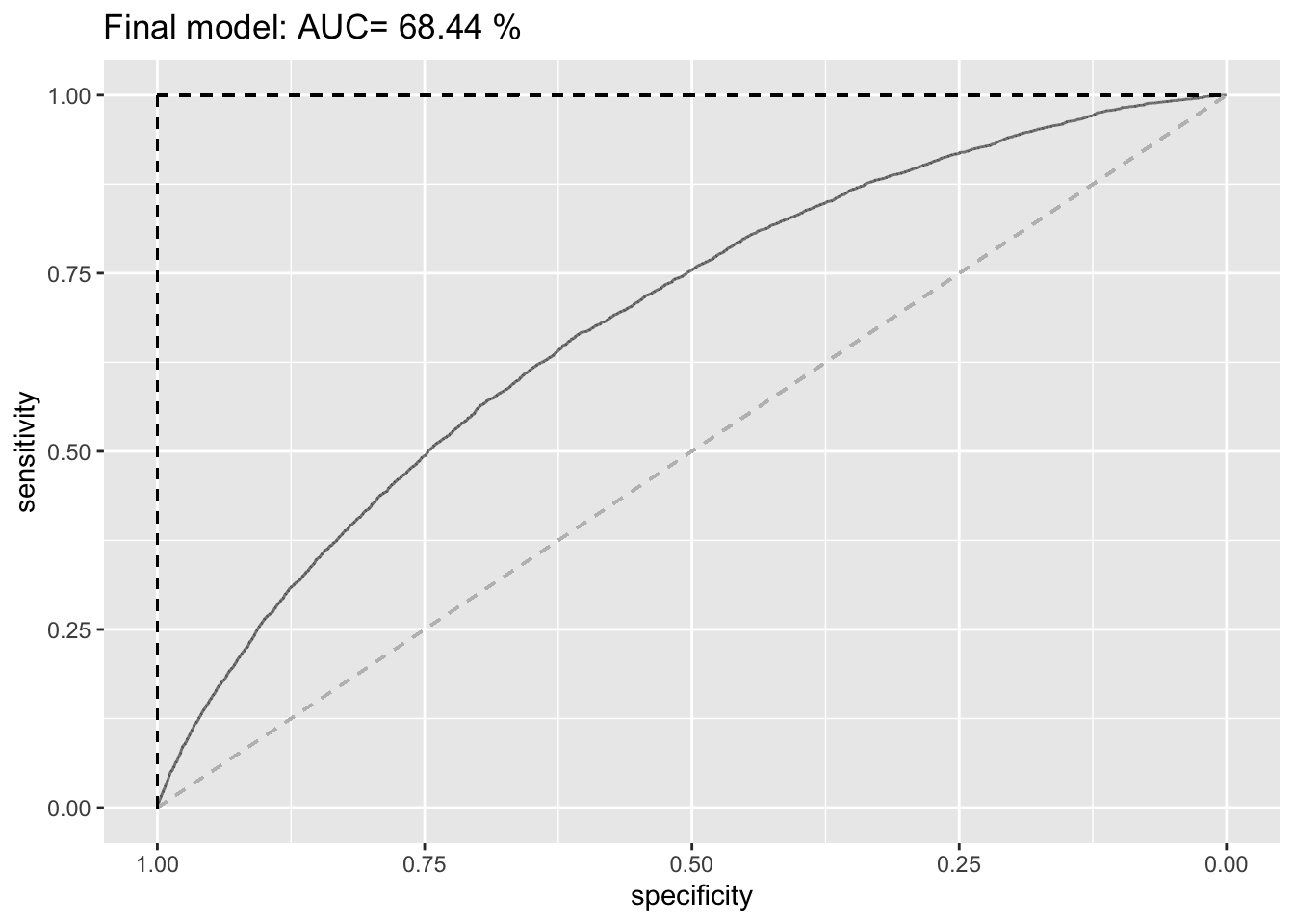

#in and out of sample testing
set.seed(4567)
train_test_split <- initial_split(lc_clean, prop = 0.8)
testing <- testing(train_test_split) #20% of the data is set aside for testing
training <- training(train_test_split) #80% of the data is set aside for training

# run finalmodel on the training set 
finalmodel_train <- glm(default ~ log(annual_inc) + loan_amnt:int_rate + term + log(int_rate):grade, family= "binomial", training)

#calculate probability of default in the training sample 
p_fm_in <- predict(finalmodel_train, training, type = "response") 

#ROC curve using in-sample predictions
ROC_fm_in <- roc(training$default, p_fm_in)

## Setting levels: control = 0, case = 1
## Setting direction: controls < cases

#AUC using in-sample predictions
AUC_fm_in <- round(auc(training$default, p_fm_in)*100, digits=2)

## Setting levels: control = 0, case = 1
## Setting direction: controls < cases

#calculate probability of default out of sample 
p_fm_out <- predict(finalmodel_train, testing, type = "response") 

#ROC curve using out-of-sample predictions
ROC_fm_out <- roc(testing$default, p_fm_out)

## Setting levels: control = 0, case = 1
## Setting direction: controls < cases

#AUC using out-of-sample predictions
AUC_fm_out <- round(auc(testing$default, p_fm_out)*100, digits=2)

## Setting levels: control = 0, case = 1
## Setting direction: controls < cases

#plot in the same figure both ROC curves and print the AUC of both curves in the title
ROC_fm_both <- ggroc(list("Final model in-sample"=ROC_fm_in, "Final model out-of-sample"=ROC_fm_out)) +
  ggtitle(paste("Final model in-sample AUC=", 
                AUC_fm_in,"%\nFInal model out-of-sample AUC=",
                AUC_fm_out,"%"))+
  geom_segment(aes(x = 1, xend = 0, y = 0, yend = 1), color="grey", linetype="dashed")+
  geom_segment(aes(x = 1, xend = 1, y = 0, yend = 1), color="black", linetype="dashed") +
  geom_segment(aes(x = 1, xend = 0, y = 1, yend = 1), color="black", linetype="dashed") +
  labs(colour = "ROC curves") +
  NULL

ROC_fm_both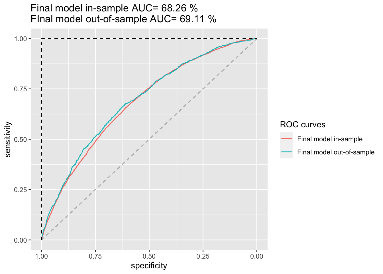

The final model includes annual_inc, loan_amnt, int_rate, term and grade in various forms of transformations and interactions. We introduce log transformations to our model as it will effectively change a unit change to a percent change and will, therefore, make the included variables better comparable (as they don’t have the same unit scales). When considering the correlation matrix, it becomes clear that some variables are somewhat correlated with each other; to account for this effect of one variable depending on the value of another variable, we also introduce interaction effects to our model (e.g. correlation between interest rate and loan amount at 0.31).

It is more complex than logistic1 and logistic2 but it yields a better goodness of fit. First and foremost, we find that the Residual Deviance is reduced to 29100 with the final model compared to a Deviance of 31005 for logistic1 and 29286 for logistic2. Moreover, the AIC of 29306 from logistic2 is further reduced to 29122 with the finalmodel. This metric (AIC) is more appropriate here as we deal with several model features. Lastly, logistic2 was able to yield an AUC of 68.01%, followed by an in-sample AUC of 68.13% and an out-of-sample AUC of 67.51%. Our final model also improves these as it yields an overall AUC of 68.44%, followed by an in-sample AUC of 68.28% and an out-of sample AUC (best among all of these) of 69.11%. Consequently, we were able to improve our out-of-sample AUC by 1.6 percentage points. Considering the in- and out-of-sample ROC curves of the final model, we can also see that our model does not suffer from overfitting.

Overall, we could have increased the general AUC to 68.45% or 68.46% as well as decreased the AIC further to 29121 by including dti and/or an interaction term between dti and annual income in our model. These are only slight improvements and the in-sample AUCs of these models would also online slightly increase; the out-of-sample AUCs of these models were however smaller than that of our final model. Considering these statistics as well as the fact that a simpler model is always better than a complex model, we conclude that our final model performs best for our purposes. While this final model is already quite complex itself, we did find that less complex models also work; their performance and especially their out-of-sample AUC is, however, far lower than that of our final model so that we stick to our final model. Using regularization through LASSO only decreased our models’ performances so that we disregard it completely.

#finalmodel_train <- glm(default ~ log(annual_inc) + loan_amnt:int_rate + term + log(int_rate):grade, family= "binomial", training)
#p_fm_out <- predict(finalmodel_train, testing, type = "response") 

testing_fm <- cbind(testing, p_fm_out)

returns_fm <- testing_fm %>% 
  mutate(
    #return if not default
    profit = installment*term_months/loan_amnt-1,
    #return if default
    loss = -0.6,
    #probability of not default
    profit_prob = 1-p_fm_out,
    #probability of default
    loss_prob = p_fm_out,
    #expected return
    expected_return = profit * profit_prob + loss * loss_prob,
    ) 

#for n = 800
returns_fm %>% 
  arrange(desc(expected_return)) %>% 
  top_n(800) %>% 
  mutate(real_return = ifelse(default == "0", (installment*term_months/loan_amnt-1),-0.6)) %>%
  summarize(
  total_exp_return = sum(expected_return),
  total_real_return = sum(real_return),
  exp_return_on_invest = (total_exp_return/800*100),
  real_return_on_invest = (total_real_return/800*100)
  )

## Selecting by expected_return

total_exp_return	total_real_return	exp_return_on_invest	real_return_on_invest
188	179	23.4	22.3

  #total_exp_return = 187.5981          
  #total_real_return = 178.7685 
  #exp_return_on_invest = 23.44976  
  #real_return_on_invest = 22.34606

Comparing the final model against logistic2 on the realized return of 800 loans chosen out-of-sample, we find that logistic2 finds a realized return of $186.50 whereas our final model finds a slightly lower realized return of $178.77.

The file “Assessment Data_2020.csv” contains information on almost 1800 new loans. We use our best model (see previous question) to choose 200 loans to invest. For this question, we assume that the loss proportion is 60%.

lc_assessment<- read_csv(here::here("data", "Assessment Data_2020.csv")) %>%  #load the data 
  clean_names() %>% # use janitor::clean_names() 
  mutate(
    issue_d = mdy(issue_d),  # lubridate::mdy() to fix date format
    term = factor(term_months),     # turn 'term' into a categorical variable
    delinq_2yrs = factor(delinq_2yrs)) # turn 'delinq_2yrs' into a categorical variable

## Parsed with column specification:
## cols(
##   `Loan number` = col_double(),
##   int_rate = col_double(),
##   loan_amnt = col_double(),
##   `term (months)` = col_double(),
##   installment = col_number(),
##   dti = col_double(),
##   delinq_2yrs = col_double(),
##   annual_inc = col_double(),
##   grade = col_character(),
##   emp_title = col_logical(),
##   emp_length = col_character(),
##   home_ownership = col_character(),
##   verification_status = col_character(),
##   issue_d = col_character()
## )

#use trained final model for predictions on lc_assessment

#finalmodel_train <- glm(default ~ log(annual_inc) + loan_amnt:int_rate + term + log(int_rate):grade, family= "binomial", training)

#predict probability of default on assessment data set
p_assess <- predict(finalmodel_train, lc_assessment, type = "response") 

lc_assessment_new <- cbind(lc_assessment, p_assess)

lc_assessment_returns <- lc_assessment_new %>% 
  mutate(
    #return if not default
    profit = installment*term_months/loan_amnt-1,
    #return if default
    loss = -0.6,
    #probability of not default
    profit_prob = 1-p_assess,
    #probability of default
    loss_prob = p_assess,
    #expected return
    expected_return = profit * profit_prob + loss * loss_prob
    ) 

#top 200
#lc_assessment_returns %>% 
#  arrange(desc(expected_return)) %>% 
#  top_n(200) 

#calculate the minimum expected return of our top 200 loans
min_return <- lc_assessment_returns %>% 
  arrange(desc(expected_return)) %>% 
  top_n(200) %>% 
  summarize(min_return_value = min(expected_return))

## Selecting by expected_return

min_return # = 0.1906794

min_return_value
0.191

#create excel input
excel_input <- lc_assessment_returns %>% 
  summarize(loan_number = loan_number,
            marie_cordes = ifelse(expected_return >= as.numeric(min_return), 1, 0))

#create excel
write.csv(excel_input, "marie_cordes.csv", row.names = FALSE)

Critique

No data science engagement is perfect. Before finishing a project is always important to reflect on the limitations of the analysis and suggest ways for future improvement.

We provide a critique of our work. What would we want to add to this analysis before we use it in practice?

Generally, the final model chosen is rather complicated. While its goodness of fit increases compared to the previous models (logistic1 and logistic2), its complexity also increases significantly. Therefore, it would be helpful to find either a model that may be complex but increases the performance by a much more significant share than the final model does now (e.g. AUC of 75% and above) or a model that is very simple but still reaches a similar out-of-sample AUC of around 69%. Potential additions/changes to the model are:

Different features: Adding or changing the features used. While exploring models, we found that dti can also help to improve the model’s performance. Further variables that may improve the model could be installment or perhaps home_ownership or verification_status. Playing around with additional features and different feature combinations from the lc_clean data set as well as introducing/changing further transformations and interaction terms for these variables may further improve the model’s performance.
Additional data: This analysis is only focused on the internal Lending Club data. It may, however, be helpful to take external factors of the macroeconomic environment into account. When exploring different models, we found that both consumer index prices as well as inflation data does not contribute to our model. Nevertheless, other information such as, for example, data on the S&P 500 returns may improve the model’s predictions as it includes external factors from the economy that influence a loan-taker’s ability to fully pay back a loan or not (default or not).
Different methods: Perhaps, using a regularization or using different split shares for our in and out of sample regressions could improve our model further if done correctly.
Standardization: As we use different variables with very different unit scales, we may find that a particular feature dominates the others in the logistic regression as its unit scale is the largest. As an improvement to our model, we could normalize/standardize all variables to the same scale to make them more comparable and use them as equally weighted features in the model.

In our analysis we did not use information about the applicants race or gender. Why is that the case? Should we have done?

We don’t use information on loan applicants race or gender to ensure that our predictions are fair and non-discriminatory. While algorithms like our model here are increasingly used and helpful to make decisions on e.g. how to reduce costs, improve efficiency or enhance customer personalization, they still pose a risk of reinforcing discriminatory behaviour in which certain groups are preferred over other groups based on their race or gender. To not accentuate possible inequalities in a society, we ensure that our model does not reinforce such discriminatory biases but rather provides financial inclusion. Therefore, and to maintain fairness in our predictions, we do not include information on race or gender. This way, our predictions of loan default are not subject to aloan holders’ race or gender, eliminating (illegal) discriminatory biases and providing inclusive and fair results.